This paper aims to shed light on the factors that shape the distribution of firm growth and on what role policies play in driving cross-country differences.
Nesta Working Paper 14/03
Issued: March 2014
JEL Classification: D92, L11, O49
Keywords: growth, firm dynamics, productivity
Abstract
Notwithstanding the growing body of evidence documenting large cross-country differences in firm growth dynamics, our understanding of what drives them is still rather limited. This paper seeks to help close this gap. Using unique data for ten countries the analysis sheds light on the factors that shape the distribution of firm growth and on what role policies play in driving cross-country differences. The paper provides new evidence on the link of labour market regulation, bankruptcy legislation, financial market development and R&D support policies with growth dynamics. The study goes beyond looking at differences in average growth rates as it analyses changes in the whole distribution of firms.
The results show that financial development, higher banking competition and better contract enforcement are associated with a more dynamic growth distribution, with a lower share of stable firms and higher shares of growing and shrinking firms, and with a more rapid expansion and contraction at the extremes of the growth distribution. Stringent employment protection legislation, as well as generous R&D fiscal incentives, are associated with a less dynamic firm growth distribution, with more stable firms and fewer growing and shrinking firms. The direction of the link between bankruptcy regime and growth dynamics is less clear-cut and varies according to the capital intensity and the dependence on external finance of the sector considered.
Authors
Albert Bravo-Biosca, Chiara Criscuolo, Carlo Menon
Albert Bravo-Biosca Chiara Criscuolo Carlo Menon
Nesta Working Paper 14/03 March 2014 www.nesta.org.uk/wp14-03
Abstract
Notwithstanding the growing body of evidence documenting large cross-country differences in firm growth dynamics, our understanding of what drives them is still rather limited. This paper seeks to help close this gap. Using unique data for ten countries the analysis sheds light on the factors that shape the distribution of firm growth and on what role policies play in driving cross-country differences. The paper provides new evidence on the link of labour market regulation, bankruptcy legislation, financial market development and R&D support policies with growth dynamics. The study goes beyond looking at differences in average growth rates as it analyses changes in the whole distribution of firms. The results show that financial development, higher banking competition and better contract enforcement are associated with a more dynamic growth distribution, with a lower share of stable firms and higher shares of growing and shrinking firms, and with a more rapid expansion and contraction at the extremes of the growth distribution. Stringent employment protection legislation, as well as generous R&D fiscal incentives, are associated with a less dynamic firm growth distribution, with more stable firms and fewer growing and shrinking firms. The direction of the link between bankruptcy regime and growth dynamics is less clear-cut and varies according to the capital intensity and the dependence on external finance of the sector considered.
JEL Classification: D92, L11, 049 Keywords: growth, firm dynamics, productivity
The authors would like to thank Dan Andrews, Javier Miranda, Dirk Pilat, Mariagrazia Squicciarini and Andrew Wyckoff for very useful discussions and comments. We are also grateful to the members of the OECD Committee for Innovation, Industry and Entrepreneurship (CIIE) and its Working Party on Industry Analysis for very valuable comments. This research was started when Albert Bravo-Biosca was a visiting economist at the OECD. The data used in this paper would not exist without the generous collaboration of many researchers and statistical agencies in the countries that participated in the Nesta-FORA firm growth project: Werner Hölzl (Austria), Sonja Djukic, Chris Johnston and Chris Parsley (Canada), Henrik Lynge Hansen (Denmark), Henri Kahonen, Petri Rouvinen and Mika Pajarinen (Finland), Stavroula Maroulaki and Theano Tyfoxylou (Greece), Patrizia Cella and Caterina Viviano (Italy), Rico Konen (Netherlands), Geoff Mead (New Zealand), Svein Myro and Christian L. Wold Eide (Norway), Valentín Llorente Garcia (Spain), Michael Anyadike-Danes and Mark Hart (United Kingdom), and David Brown and Javier Miranda (United States). Chiara Criscuolo, OECD, 2 rue André Pascal, 75775 Paris Cedex 16, France. Email: [email protected]
The Nesta Working Paper Series is intended to make available early results of research undertaken or supported by Nesta and its partners in order to elicit comments and suggestions for revisions and to encourage discussion and further debate prior to publication (ISSN 2050-9820). © Year 2014 by the author(s). Short sections of text, tables and figures may be reproduced without explicit permission provided that full credit is given to the source. The views expressed in this working paper are those of the author(s) and do not necessarily represent those of Nesta.
- 1. Executive summary
- 2. Introduction
- 3. Data
- 4. Regression analysis
- 4.2. Interactions between industry characteristics and policies and framework conditions
- 5. Results
- Table 7, column 1 explores the impact of more severe bankruptcy regimes on multifactor productivity (MFP). The estimates show that in capital intensive industries and in industries where minimum efficient scale is lower tighter bankruptcy regimes are associated with lower MFP growth. In the latter sectors and in sectors that are R&D intensive, tighter bankruptcy regimes
- 5.5. Regressions with multiple interactions terms, robustness and unreported results
- 6. Conclusions
- REFERENCES
- ANNEX A
- ANNEX B:
- ANNEX C: OLS RESULTS
- APPENDIX
- 1.2. OECD-ORBIS 2011 database
- II. OECD-ORBIS 2011 vs. Nesta-FORA firm growth project
- III. Concluding remarks
1. Executive summary
Firm employment dynamics are at the core of policy discussions on jobs and productivity. A growing body of evidence shows large differences in job creation and destruction across countries. However, our understanding of the drivers of employment dynamics is limited, hampering policy development.
Most existing analysis has focused on partial evidence of firm employment dynamics such as average employment growth; the share of high-growth firms; or the entry and exit of firms. While useful, this analysis does not shed much light on firms' heterogeneous responses to the same exogenous shock nor on the heterogeneous impact of policies and framework conditions across different firms, even within the same sector.
This paper exploits recently available harmonised aggregated micro-data on firm growth dynamics in both manufacturing and non-manufacturing sectors to explore what drives the dynamics of business growth across ten OECD countries. The data describes the whole distribution of firm employment growth, and so it captures the heterogeneity of firm growth dynamics within sectors.
More specifically, the data provides measures for the percentiles of the growth distribution for surviving firms during 2002-2005, as well as the share of firms growing or shrinking at a particular rate (up to 11 categories such as high, medium, low or negative growth). It shows clear differences in the process of resource reallocation across countries, with the United States displaying a higher level of business dynamism than most continental European economies for which data are available.
The data shows a number of empirical regularities that hold across the ten countries considered here (United States, Canada, and eight European countries: Austria, Denmark, Finland, Italy, Netherlands, Norway, Spain and the United Kingdom):
- There is a clear correlation between job expansion and job contraction; these occur simultaneously, confirming the existence of an active process of creative destruction. It also suggests that the process of creative destruction operates both at the "intensive margin" (i.e. the expansion and contraction of incumbent firms), and at the "extensive margin" (i.e. firm entry and exit).
- High-growth firms (HGFs) make a disproportionate contribution to employment growth. These firms account only for between 3.2% (Norway) and 6.4% (United Kingdom) of all surviving firms with ten or more employees, yet they account for 40% and 64% of all jobs created by surviving firms with ten or more employees in Norway and United Kingdom, respectively. However, non-HGFs still account for between a third and three-quarters of job creation, highlighting the need to consider the full growth distribution when designing policies to foster job creation.
- Growth is more volatile amongst young businesses and less so among larger and more mature businesses.
- Services and construction are much more dynamic sectors than manufacturing, with higher levels of both job creation and job destruction.
The main goal of the paper is to examine whether policies and framework conditions can help explain the observed differences in firm growth dynamics across countries. Specifically, the analysis investigates the role of regulatory and judicial frameworks (i.e. bankruptcy laws, employment protection legislation), financial market institutions, and R&D support policies (i.e. R&D fiscal incentives).
To do so, the analysis exploits a "difference-in-differences” approach that focuses on the differential impact of policies on the employment growth distribution across different sectors to control for country and industry unobservable factors. In addition, it uses an instrumental variables method to solve the endogeneity problems that arise from measurement error.
The analysis confirms that policies and framework conditions have heterogeneous impacts along the distribution of firm employment growth. In other words, the impacts of policies and framework conditions are not necessarily the same for firms characterised by low, average or high growth. As a result, policies and framework conditions also affect the overall shape of the growth distribution, measured both as the differential in growth performance of firms in the bottom and top quartile of the distribution and as the share of firms with different growth performances.
The main findings of the report are as follows:
Labour market regulation
- Inflexible labour market regulation can affect firms' willingness to take risks and experiment with uncertain growth opportunities. Stringent regulation increases the costs of downward adjustment and is likely to encourage a more conservative growth strategy (which in turns decreases the pressure on underperforming firms). Lower risk taking and slower job reallocation may in turn reduce productivity growth. Firms may be less willing to expand their workforce or enter into new markets if they cannot reduce their workforce later if their efforts prove to be unsuccessful. Therefore, inflexible labour market regulation reduces average employment growth in more innovative and thus risky/volatile industries. It may also lead to more conservative growth strategies, with slow gradual expansion rather than fast growth, in sectors where labour costs are high.
- The results show that stringent employment protection legislation leads to a less dynamic firm growth distribution. Specifically, strict EPL is associated with a higher share of stable firms (and a lower share of growing and shrinking firms) in R&D intensive sectors, which in turn leads to significantly lower productivity growth. Collective dismissals regulation is also associated with a narrowing of the growth distribution in labour intensive sectors, with firms in the bottom quartile of the distribution growing faster (or, more likely, contracting more slowly) and firms at the top of the distribution achieving lower growth.
Bankruptcy
- Bankruptcy regimes that severely penalise “failed” entrepreneurs, whether by forcing liquidation or limiting entrepreneurs' ability to start new businesses in the future, are likely to reduce their willingness to take risks. On the other hand, tight bankruptcy regulation with strong creditor rights is likely to decrease the cost of raising external finance, which helps firms to grow. Tight regulation might reassure financiers about their ability to recoup their investments in case of failure as well as reduce moral hazard and adverse selection concerns. Therefore, while a creditor-friendly bankruptcy regime may reduce the overall variance of the growth distribution, the opposite effect is also possible.
- The tightness of a bankruptcy regime impacts the shape of the growth distribution, but also reflects a trade-off between the creditors' insurance effect and strict credit conditions. On the one hand, in sectors that are relatively capital intensive and those with lower efficient scale of production, strong creditor rights are associated with a squeeze of the firm growth distribution towards the middle, with a more limited dispersion. On the other hand, in industries that are highly dependent on external finance, stronger creditor rights are correlated with a fall in the number of stable firms, so an effect going in the opposite direction.
Financial institutions
- Financial development is an important driver of economic growth and affects the reallocation of resources within and across industries. It boosts the growth of the best performing firms, since external finance is an important ingredient for firms that are aiming to grow fast. On the other hand, a more developed financial market may also provide some resources to underperforming firms, allowing them a second chance to improve their performance, and so slowing down rather than speeding up the reallocation of resources. Therefore, how financial development affects the shape of the firm growth distribution is ultimately an empirical question.
- The results suggest that more developed financial institutions are associated with a widening of the growth distribution in industries that are highly dependent on external finance, although the magnitude of the effect is not large. The widening of the distribution is driven by faster growth among the best performing firms, faster contraction of underperforming firms and a smaller share of stable firms in the middle. Regulations that encourage banking competition and an efficient judicial system to enforce contracts are also correlated with a more dynamic growth distribution.
R&D fiscal incentives
- R&D fiscal incentives are one of the tools most commonly used by governments to encourage innovation in the private sector. Their impact on the distribution of firm growth crucially depends on the direct and indirect impacts of the policy. R&D fiscal incentives might benefit relatively more established incumbents (in which case the policy would reduce the dynamism of the growth distribution), highly-innovative firms at the technology frontier (which should lead to higher dynamism) or second-rate projects in underperforming firms. They might on the other hand benefit young start-ups that do not have high tax bills relatively less.
- The analysis finds that R&D fiscal incentives are correlated with a narrower growth distribution in R&D intensive sectors, with fewer shrinking firms and more stable ones. Firms in the bottom half of the distribution contract more slowly, while firms at the top of the distribution experience lower growth. The results also suggest a negative effect on entry. This suggests that R&D support measures may have the unintended consequence of protecting incumbents and slowing down the reallocation of resources towards more innovative entrants.
Unreported results include numerous robustness checks as well as analysis of other policies such as product market regulation; barriers to entrepreneurship; barriers to trade and foreign direct investment; taxes and social contributions; political stability and corruption. These results were inconclusive, most likely due to limitations in the available data.
2. Introduction
Employment and productivity growth are at the heart of current policy discussions, yet our understanding of which policies are more effective at encouraging their growth is still limited. Growing empirical evidence confirms the role of government policies and framework conditions in explaining – at least partially – the existence of significant differences across countries in employment and productivity dynamics. However, much of the existing literature has focused on the "average firm", while firms are heterogeneous and so are their employment and productivity dynamics.
The main contribution of this paper is to fill this gap and provide new evidence on how policies and framework conditions are correlated with employment growth of firms along the whole growth distribution. Specifically, this paper aims to answer the following questions: what are the factors underlying the variations in employment growth across different countries? What are the role of framework conditions, regulatory factors and policies such as R&D support and employment protection legislation?
Recent evidence suggests that firm dynamics are important for processes of creative destruction, selection and learning that underlie aggregate employment and productivity growth (OECD, 2009b, Bartelsman et al., 2009a and Bravo-Biosca, 2010b). While much of the variation in firm churning rates is explained by differences in sectoral composition, differences in the post-entry performance of firms remain even after controlling for sectoral effects. It is therefore likely that they reflect the role of differences in countries' policies, market structures and institutional frameworks.
The report extends the existing literature in a number of ways. Most existing research focuses on the impact of policies and framework conditions on average employment and productivity growth on the one hand and on entry and exit of firms on the other (i.e. the so-called “extensive margin"). Thus far, none of the cross-country studies has looked at how policies and framework conditions have affected growth at different points in the growth distribution, nor have they investigated how they have affected the shape of the growth distribution.
This paper explores the heterogeneous impact of a set of policies and institutions on post-entry employment growth across firms. It complements the nascent literature on high-growth firms and how policies can support them. However, instead of focusing on only one part of the employment growth distribution, the top performers, it also considers firms with medium, low or negative growth. Looking at the whole distribution conveys a fuller picture of the impacts of policies on employment growth across different groups of firms.
The analysis exploits recently available harmonised aggregated micro data on firm growth dynamics in both manufacturing and non-manufacturing sectors (Bravo-Biosca, 2010b) to explore what drives the dynamics of business growth across ten countries (the United States, Canada, and eight European countries: Austria, Denmark, Finland, Italy, Netherlands, Norway, Spain and the United Kingdom).1 The data used here focuses on the intensive margin of the job reallocation process through expansion and contraction (i.e. on incumbent firms' employment growth) during the 2002-2005 period. The data shows several interesting empirical regularities and patterns across different groups of firms that hold across countries, which are consistent with the available evidence from single country analyses and at European level.
The analysis investigates the role of differences in policies and framework conditions using a "difference-in-differences” approach combined with an instrumental variables estimation to correct for possible biases due to measurement error problems. This methodology provides comparative evidence on the differential impact of policies and institutions at different points of the growth distribution, controlling for country and industry unobservable factors.
The paper focuses on four policy areas: employment protection legislation, financial market development, bankruptcy laws and R&D fiscal incentives. The results show that these have a heterogeneous impact across the distribution of firm employment growth and affect its overall shape, measured both as the growth gap between the bottom and the top quartile of firms and the share of firms in different brackets of growth performance. Specifically, the following conclusions emerge:
- Tight employment protection legislation (EPL) is associated with a more static employment growth distribution in R&D intensive sectors, with a lower share of growing and shrinking firms and a larger number of stable firms. In light of existing evidence, the results also show that stringent EPL is correlated with lower multifactor productivity growth (MFP) in R&D intensive sectors. Collective dismissals regulation is also associated with a narrower growth distribution in labour intensive sectors.
- Bankruptcy regimes have an impact on the distribution of firm growth, which reflects the trade-off between incentivising risk-taking by firms and entrepreneurs on the one hand, and increasing access to credit through stronger investors' protection on the other. Creditor-friendly regimes are correlated with lower dynamism in capital intensive sectors and in sectors with low technological barriers to entry. However, they are also correlated with a more dynamic growth distribution in industries with a high dependence on external finance.
- Financial development is associated with higher dynamism in industries that are highly dependent on external finance, although the magnitude of the effect is not large. Top performing firms grow faster, underperforming firms contract faster, and fewer firms remain stable. Regulation that encourages banking competition and an efficient judicial system to enforce contracts are also correlated with a widening of the growth distribution.
- R&D fiscal incentives are associated with a less dynamic growth distribution in R&D intensive sectors, with significantly fewer shrinking firms and more stable firms. Firms at the top of the distribution grow more slowly, while firms in the bottom half do not shrink as fast.
The report is organised as follows: the next section presents the different data sources used in the analysis. Section 3 discusses the methodology used. Section 4 reports the results of the analysis and relates them to the existing evidence. Finally, Section 5 summarises the evidence and concludes. The Annexes include details on the variables used and additional results. A final Appendix provides a comparison of firm growth indicators obtained from commercial databases vs. business registers.
3. Data
The empirical analysis in this paper exploits a rich database which combines aggregated data on the distribution of firm growth at industry and country level, information at country level on a wide spectrum of national policies and characteristics of the business environment, and a number of industry-specific variables reflecting the technological characteristics of sectors.
3.1 Data on firm growth
This paper uses a novel database on the distribution of firms' growth that was collected as part of a joint project by FORA and Nesta in collaboration with researchers and national statistical agencies in 12 countries and with support from the International Consortium for Entrepreneurship (ICE) and the Entrepreneurship Indicators Programme (EIP) of the OECD. The following description and discussion of the database draws extensively on Bravo-Biosca (2010b), which contains additional information.
Measuring the distribution of business growth consistently across countries is challenging. There are currently two different data sources to accomplish this task, standard commercial databases and business registers.
Several studies have used commercial databases, such as Bureau van Dijk's ORBIS, which typically collect data from companies' fillings and yellow pages directories (see OECDb 2009). However, the coverage of business activity in commercial databases is limited and differs across countries, over time, and across size classes, being better for larger businesses (see the Entrepreneurship Indicator Programme at the OECD and Ragoussis and Gonnard, 2012 for more details2). This creates problems of data comparability when conducting cross-country analysis as in this paper. The Appendix provides a more detailed comparison of firm growth indicators obtained from business registers and the ORBIS database.
Business registers collect information on firms' entry, exit, and employment and/or turnover from social security records, tax records, censuses and/or other administrative sources. Therefore, they provide the most comprehensive coverage of economic activity in any country, basically covering the universe of firms. However, due to the confidential nature of the information, access to this rich data source is restricted.
To circumvent confidentiality, Bravo-Biosca (2010b) built a micro-aggregated database on firm growth dynamics with information from business registers, following the approach used by other researchers (Bartelsman, Haltiwanger and Scarpetta 2004, Brandt 2004, OECD 2009a). The database is based on a partnership with each country's national statistical offices or, alternatively, with researchers that have authorised access to the microdata. Participants were provided with a methodological manual and software code to extract the required data, building – whenever feasible – on the Eurostat-OECD Business Demography Manual (2007), which most business registers follow. The information submitted by each partner was then scrutinised to identify potential inconsistencies and, if necessary, subjected to a process of revisions with each partner in the project.
Collaborations were established across twelve countries: Austria, Canada, Denmark, Finland, Greece, Italy, the Netherlands, New Zealand, Norway, Spain, the United Kingdom and the United States. Each country provided harmonised micro aggregated data on business growth following standard definitions provided at the outset of this project, which in turn were based on the Eurostat-OECD Manual on Business Demography Statistics developed by the Entrepreneurship Indicators Programme. The resulting database draws on individual records for six million firms, which employed over 120 million people in 2002. It measures how firms expanded and shrank between 2002 and 2005: the period after the dotcom bubble and before the height of the boom that later degenerated into the recent financial crisis (data is also available for some countries up to 2008).
Average annual employment growth over a three-year period was measured for each surviving private sector firm that had at least one employee and was at least one year old (turnover growth data is also available for some countries). Based on their growth rate, firms were placed in one of 11 pre-defined growth intervals.3 This data was then used to estimate the percentiles of the growth distribution and produce a growth distribution curve for each country.4 The resulting database contains the full growth distribution and a variety of other indicators on business growth for up to 51 sectors, ten firm size classes and five age groups in 12 countries. The data used in the analysis is, however, restricted to ten countries (Austria, Canada, Denmark, Finland, Italy, the Netherlands, Norway, Spain, the United Kingdom and the United States) and 36 sectors.
A few issues regarding the database are worth being highlighted. First, the growth data for the United Kingdom was derived from a database still under development, so changes may occur in future revisions. Second, the data for Canada only covers firms with between 10 and 250 employees. Third, the data only includes surviving firms (defined as those that have survived with positive employment throughout the three-year period); therefore the data does not allow for the analysis of entry and exit patterns, or for the contribution of entry and exit to aggregate employment growth. Fourth, data was collected for all firms with at least one employee, but the firm growth indicators discussed here focus on firms with ten or more employees, since percentage growth rates for very small firms are often very “noisy” indicators (e.g. a firm growing from two to four employees has a 100% employment growth rate). Fifth, the breakdown for age and size categories is not available at the 2-digit industry level but only for more aggregated sectoral groupings. This means that it is not possible to distinguish in the regression analysis for factors that might affect young versus mature firms or small versus large businesses differently. Finally, all measures of job creation discussed here capture in principle all jobs gained by surviving firms, regardless of whether they are the result of organic growth or instead are gained through acquisitions of existing firms. Similarly, job destruction captures both jobs lost by firms that dismiss employees and spinouts that reduce the headcount of the firm. These measures thus capture the restructuring process that firms undertake, regardless of whether this is achieved through acquisitions, spinouts or organic growth.
Another issue relates to the boundaries of firms. The administrative or legal definition of an enterprise (or establishment) used by business registers does not necessarily coincide with the economic definition of the firm (which itself is also often diffuse). For instance, a new subsidiary of a larger firm is generally coded as a new entering firm. Shifting of activities from one plant to another is treated differently if the plants belong to the same subsidiary or to two different subsidiaries of the same firm. Outsourcing to an external provider decreases employment growth (but not turnover growth). Employment outside the home country is not measured in business registers, so FDI or offshoring are not properly captured. However, these concerns should not be over-emphasised, since the boundaries of the firm are relatively clear for the majority of firms. After all, as Bartelsman, Scarpetta and Schivardi (2003) point out, the average number of plants per firm is 1.2 in the United States and 1.1 in Finland, despite the large difference in country size.5
3.2. Exploratory descriptive analysis
This section presents a few of the findings that emerge from this novel firm growth database, which are discussed in more detail in Bravo-Biosca (2010b, 2011). The main feature of the database is the ability to explore the remarkable differences in the distribution of firm employment growth among the countries under analysis. The graphs in Figure 1 split firms in each country into 11 categories, each representing a growth interval going from firms that shrink at an average annual rate of more than 20% to high-growth firms that grow more than 20%. The resulting growth distributions look reasonably symmetric, which suggests that higher shares of high-growth firms are linked to a larger number of shrinking businesses.
Figure 1. Share of firms by growth bracket and country, firms with 10 or more employees
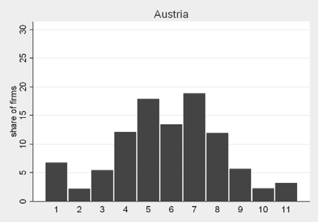
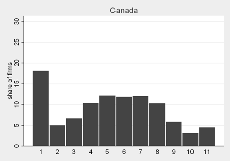
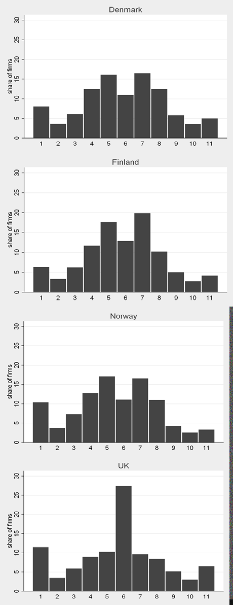
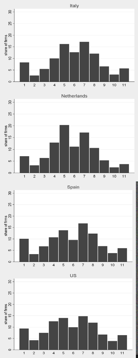
Note: the bars correspond to the share of firms relative to the total number of surviving firms in the country (with ten or more employees) with annual average employment growth over a three-year period falling within each of the following eleven growth intervals: 1: [-∞;<-20%[; 2: [-20%;-15%[; 3: [-15%;-10%[; 4: [-10%;-5%[; 5: [-5%;-1%[; 6: [-1%;+1%[ ; 7: [+1%;+5%[; 8: [+5%;+10%[; 9: [+10%;+15%[; 10: [+15%;+20%[; 11: [+20% ; + ∞]. Data for the United Kingdom are preliminary. Source: Nesta-FORA firm growth project.
The results clearly show different patterns of dynamics across countries. Figure 2 summarises these differences amongst European countries and the United States. As seen in the bottom graph, the European countries included in the sample have a larger share of stable firms (those in the middle 3 intervals, growing between -5 and 5% a year) relative to the United States where firms that grow more than 5% or shrink more than 5% a year are more prevalent. This figure highlights the strong dynamism of the United States economy relative to European countries. This result is also robust to controlling for the underlying differences in the industrial and size structure of the economies considered, and it also holds for most European countries when considered individually (Bravo-Biosca 2010a, 2011). The aim of this paper is to shed some light on some of the policies that may play a role in explaining these patterns.
Figure 2. Share of firms by growth bracket, Europe-United States comparison
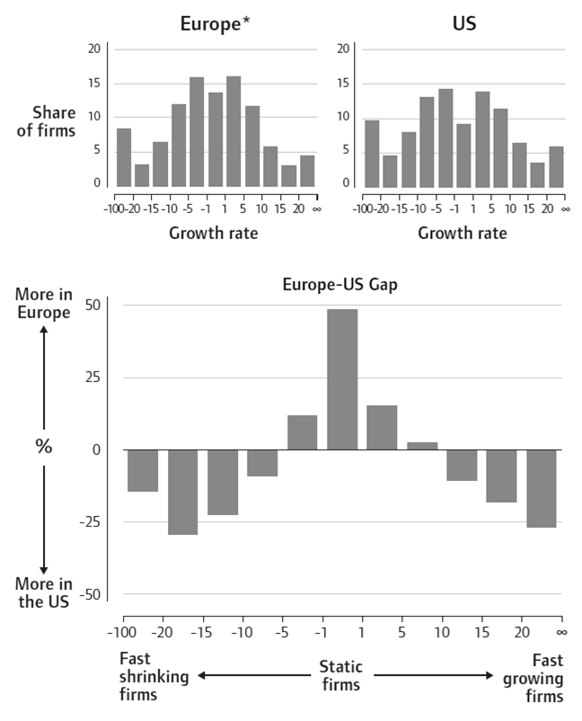
Note: Europe corresponds to the average for the European countries (Austria, Denmark, Italy, Netherlands, Spain, Norway and the United Kingdom) that participated in the Nesta-FORA firm growth project. Source: Bravo-Biosca (2011).
Figure 3 compares the distribution across countries using a more aggregate classification into four growth intervals: shrinking, stable, growing and high-growth firms. The graph sorts from left to right countries that have the lowest share of high-growth firms. These are all continental European countries: Finland, Italy, Denmark, Netherlands, Austria, and Norway. They are also the countries where the share of stable firms is the largest.
Figure 3. Share of firms by country, firms with 10 or more employees
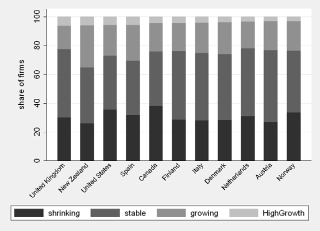
Note: Decreasing, stable, growing and high-growth firms are defined according to the following growth rate intervals, respectively: [-∞;-5%[, [-5%;+5%[, [+5%;+20%,[+20%;+∞]. All data refer to firm with 10 employees or more. Source: Nesta-FORA firm growth project.
As a result, there are large differences in the patterns of job expansion and contraction across countries. Figure 4 shows that European countries typically have lower rates of both job creation and destruction, while countries like the United States and Canada that have an above-average share of high-growth firms also have significantly larger job destruction. This confirms the importance of looking at the whole distribution of firms to understand the dynamics of employment growth rather than restricting the analysis to HGFs.
8Decreasing, stable, growing and high-growth firms are defined according to the following growth rate intervals, respectively: [-∞;-5%[, [-5%;+5%[, [+5%;+20%,[+20%;+∞]. Unless otherwise stated, all growth rate data refers to firms with 10 employees or more.
Figure 4. Share of job creation and destruction by surviving firms, by country
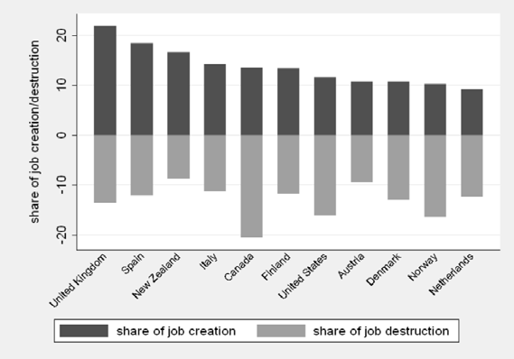
Note: The graph reports the share of jobs created and destroyed by surviving firms in the 2002-2005 period in total initial employment. All data refer to firms with 10 employees or more. Source: Nesta-FORA firm growth project.
Figure 5 reports the share of high-growth firms (HGFs), their share in total employment, and their contribution to job creation. In all countries, high-growth firms account for a very small share of the total number of firms and initial employment, but make a disproportionate contribution to job creation.
For instance, in the United Kingdom, United States, and Italy, HGFs account for more than 40% of total job creation by surviving firms with 10+ employees, while they represent on average only 5% of the total number of surviving firms with 10+ employees. Specifically, they account for between 3.2% (Norway) and 6.4% (United Kingdom) of all surviving firms with ten or more employees, yet they account for 40% and 64% of all jobs created by surviving firms with ten or more employees in Norway and United Kingdom, respectively. This justifies the prominence of high-growth firms in the debate about job creation and employment growth, although it leaves between 36% and 74.5% of employment growth to be attributed to other firms. Therefore it is important to look beyond HGFs and explore the full growth distribution. The data also allows exploring some of these empirical regularities at the 2-digit industry level. Figure 6 shows that high-growth firms make a large contribution to job creation across most sectors, although there are some differences across them. Services and construction display more concentrated job creation, with as much as 60% of sectoral employment growth being accounted for by HGFs in service sectors such as computer and related activities (Sector 72) and other business services (Sector 74).
Figure 5. Share of high-growth firms and their contribution to job creation, by country
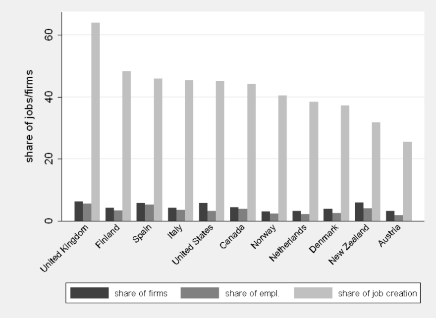
Note: High growth firms (HGFs) are enterprises with ten or more employees in the beginning of the observation period with average annualised employment growth greater than 20% over a three-year period (2002-2005). Share of firms corresponds to the share of HGFs in the total number of surviving firms in the country with ten or more employees at the beginning of the period; share of employment corresponds to the share of employment of HGFs in the aggregate employment of surviving firms with 10 employees or more at the beginning of the period; share of job creation corresponds to the share of jobs created by high-growth firms relative to all jobs created by surviving firms with ten or more employees during the three-year period 2002-2005. Source: Nesta-FORA firm growth project.
Figure 6. Share of high-growth firms and their contribution to job creation, by sector
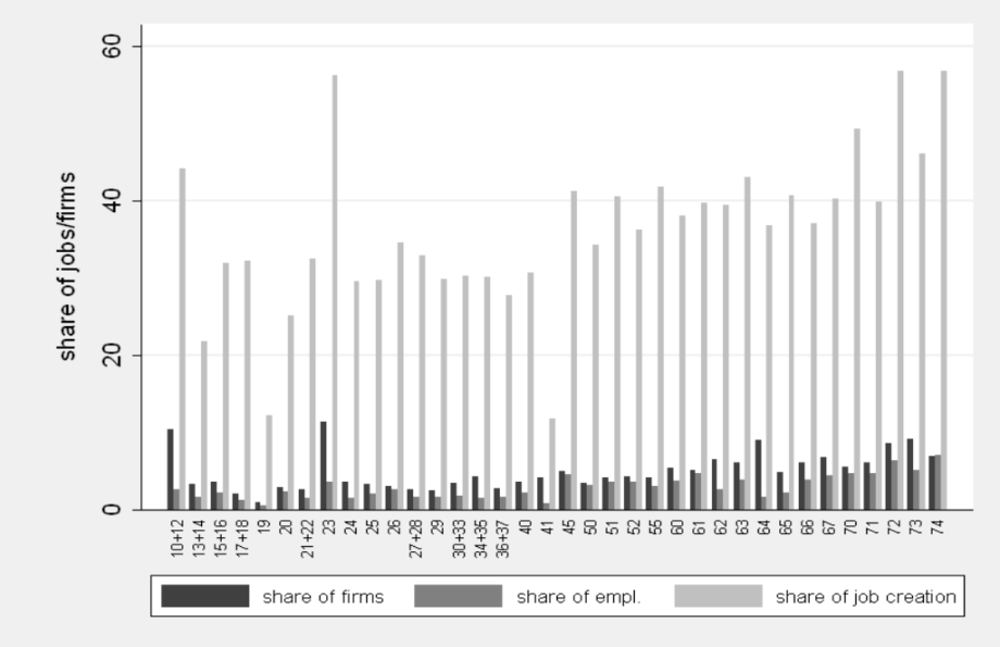
Note: High growth firms (HGFs) are enterprises with ten or more employees at the beginning of the observation period with average annualised employment growth greater than 20% over a three-year period (2002-2005). Share of firms corresponds to the share of HGFs in the total number of surviving firms in the country with ten or more employees at the beginning of the period; share of employment corresponds to the share of employment of HGFs in the aggregate employment of surviving firms with 10 employees or more at the beginning of the period; share of job creation corresponds to the share of jobs created by high-growth firms relative to all jobs created by surviving firms with ten or more employees during the three-year period 2002-2005. Industry averages are not weighted (each industry in each country has equal weight). The countries included in the graph are Austria, Denmark, Finland, Italy, Netherlands, Norway, Spain, the United Kingdom, and the US. The sectoral classification follows the ISIC 3.1 standard classification (see also http://unstats.un.org/unsd/cr/registry/regcst.asp?Cl=17) Source: Nesta-FORA firm growth project.
Significant differences across sectors also emerge when considering job creation and destruction at the 2-digit industry level, with services displaying a much more active process of resource reallocation than manufacturing sectors (Figure 7). However, while the sectoral composition matters, there are important differences in resource reallocation across different countries even after controlling for the industry structure.
Figure 7. Share of job creation and destruction by surviving firms, by sector
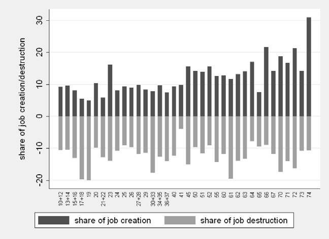
Note: The graph reports the share of jobs created and destroyed by surviving firms in the 2002-2005 period in total initial employment. All data refer to firms with 10 employees or more. The countries included in the graph are Austria, Denmark, Finland, Italy, Netherlands, Norway, Spain, the United Kingdom, and the United States. The sectoral classification follows the ISIC 3.1 standard classification (see also http://unstats.un.org/unsd/cr/registry/regcst.asp?Cl=17) Source: Nesta-FORA firm growth project.
To examine this active process of job reallocation in more detail, Figure 8 reports the correlation between job creation by HGFs (horizontal axis) and job turnover in the sector (vertical axis, defined as the sum of the shares of job expansion and job contraction in total employment) after having controlled for country and sectoral effects. In the scatter plot, every dot is a country-industry pair. There is a clear positive relationship between the intensity of job turnover and the share of jobs created by HGFs, which holds even after controlling for country and industry idiosyncratic effects. Figure 9 shows that the relationship is also positive when considering job destruction. In other words, a greater importance of high-growth firms is typically associated with faster job creation and faster job destruction. This confirms that the process of creative destruction operates both on the “intensive margin” (i.e. the expansion and contraction of incumbent firms) as well as the much studied “extensive margin” (i.e. firm entry and exit).
Figure 8. Share of job turnover and share of job creation by high-growth firms, by country/sector
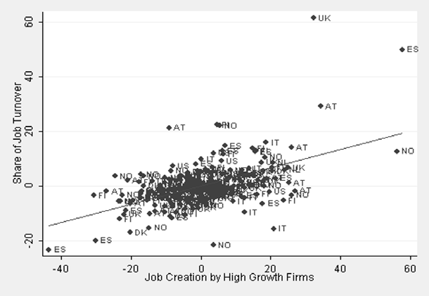
Note: The dots report of the share of job turnover (vertical axis) and jobs created by high-growth firms (those with a yearly growth rate >20%) (horizontal axis) in the period 2002-2005 in total initial employment. In order to account for country and industry effects, the graph reports the residuals of an OLS regression of the actual values on country and industry fixed effects. All data refer to firms with 10 employees or more. The countries included in the graph are Austria, Denmark, Finland, Italy, Netherlands, Norway, Spain, the United Kingdom, and the United States. Source: Nesta-FORA firm growth project.
Figure 9. Share of job destruction and share of job creation by high-growth firms, by country/sector
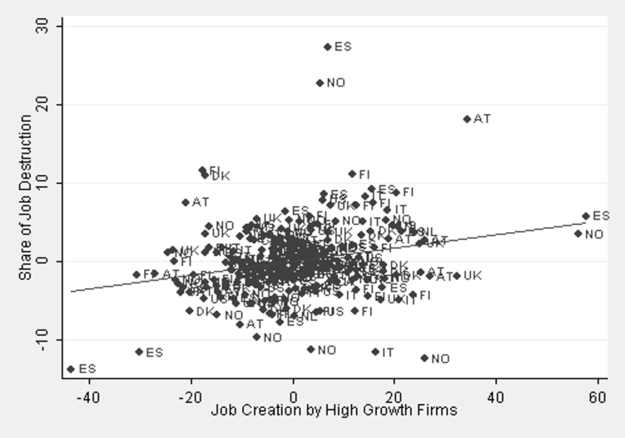
Note: The dots report of the share of jobs destroyed (vertical axis) and created (horizontal axis) by surviving firms in the period 2002-2005 in total initial employment by surviving firms. In order to control for country and industry effects, the graph reports the residuals of an OLS regression of the actual values on country and industry fixed effects. All data refer to firms with 10 employees or more. The countries included in the graph are Austria, Denmark, Finland, Italy, Netherlands, Norway, Spain, the United Kingdom, and the United States. Source: Nesta-FORA firm growth project.
Figure 10. Share of firms by age and size
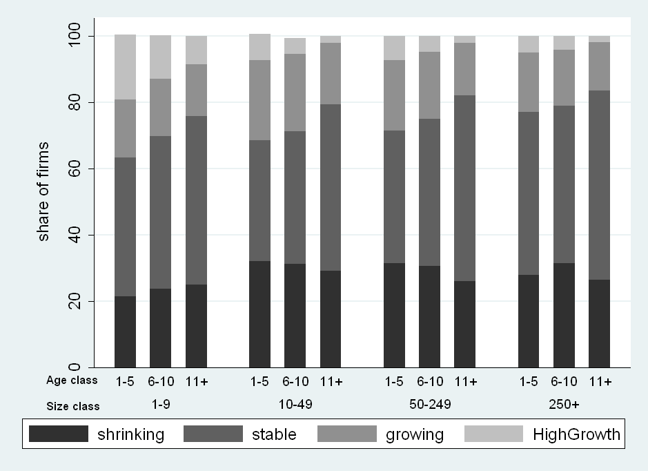
Note: Shrinking, stable, growing and high-growth firms are defined according to the following yearly growth intervals, respectively: [-∞;-5%[, [-5%;+5%[, [+5%;+20%[, [+20%;+∞]. Firms are classified in 12 groups based on the combination of 3 age classes (1-5, 6-10, 11+) and 4 size classes (1-9, 10-49, 50-249, 250+). The countries included in the graph are Austria, Denmark, Finland, Italy, Netherlands, and Norway. Source: Nesta-FORA firm growth project.
The size and the age of firms are two of the most common firm's characteristics considered in the policy debate. Figures 10 and 11 examine the firm growth distribution and the patterns of job reallocation splitting firms by their age and size profile, considering three age classes (1-5, 6-10, and 11 years or more) and four size classes (1-9, 10-49, 50-249, 250 employees or more).
Young firms display higher levels of dynamism, regardless of their size. Firstly, young firms are more likely to be high-growth than more mature firms (Figure 10). Secondly, firms younger than 11 years also display more turbulence, as shown by the smaller share of stable firms in these categories (Figure 10) and the greater job creation and job destruction rates amongst younger firms (Figure 11). Both of these features are consistent with Haltiwanger et al. (2012), who use US census data to show that young firms, rather than small firms contribute more proportionally to aggregate employment growth. However, they also show that there are “up or out” dynamics; only few of these young firms survive and grow (going “up”) while many shrink and leave the market (going "out").
Figure 11. Share of job creation and destruction by surviving firms, by age and size class
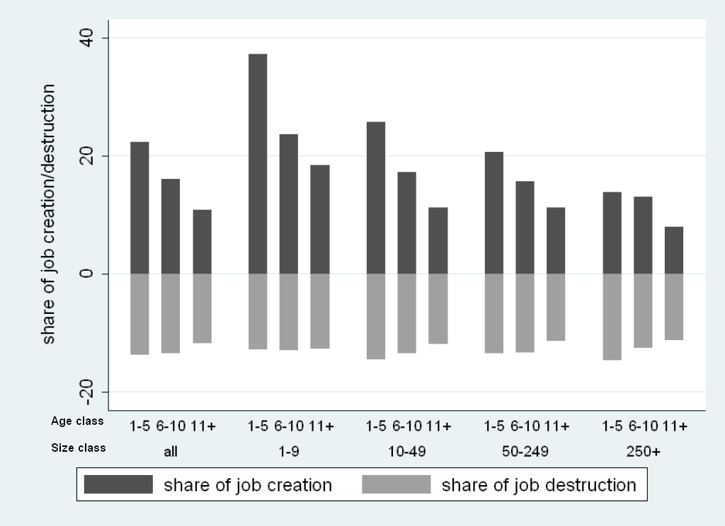
Note: The graph reports on the share of jobs created and destroyed by surviving firms in the period 2002-2005 in total initial employment. Firms are classified in 12 groups based on the combination of 3 age classes (1-5, 6-10, 11+) and 4 size classes (1-9, 10-49, 50-249, 250+). The countries included in the graph are Austria, Denmark, Finland, Italy, Netherlands, and Norway. Source: Nesta-FORA firm growth project.
The period of analysis covered by this data is limited (2002-2005), so it does not allow controlling for potential business cycles effects. Using data derived from the STAN database held at the OECD, Figure 12 shows that most participating countries experienced moderate employment growth in 2002-2005. With the exception of the Netherlands, Denmark, and the United Kingdom, aggregate employment growth rates during this period were positive, with Spain experiencing a period of exceptionally high employment growth.
The comparison with the firm growth database, which only considers growth by surviving firms that are at least one year old and thus ignores entry and exit, is instructive. Figure 13a displays the average 3-year employment growth rate for surviving firms with 1+ employees, while Figure 13b restricts the sample to surviving firms that have at least 10 employees at the beginning of the period.
The difference between Figure 12 and 13 thus provides some information on the contribution to employment growth from entry and exit. For instance, it shows that even though their economy was doing very well, United States and Norwegian incumbent firms were contracting on average. This highlights the positive contribution to employment growth from entry and exit and from growth of firms with less than 10 employees for the United States and Norway. Specifically, they go from having positive growth rates when considering the whole population of firms, including entrants and exits (Fig. 12), to having negative growth rates when restricting the sample to surviving firms, which worsens when excluding firms with less than 10 employees (Fig. 13 a and b).9
Figure 12. 3-years employment growth rate, all firms, by country
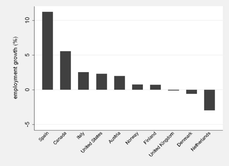
Note: The graph shows the average 3-years growth rate of employment of all firms, including entrants and exits, over the period 2002-2005. Source: OECD STAN database.
Figure 13. 3-years employment growth rate: (a) all surviving firms (b) surviving firms with more than 10 employees, by country
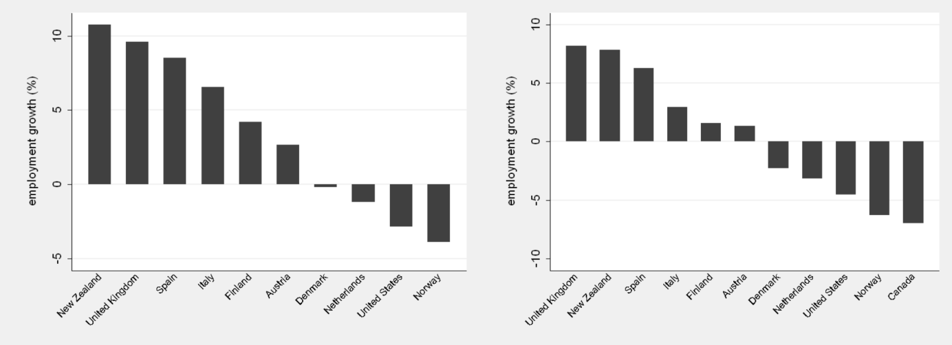
Note: (a) The graph shows the 3-years growth rate of employment of surviving firms over the period 2002-2005. (b) The graph shows the 3-years growth rate of employment of surviving firms with more than 10 employees over the period 2002-2005. Source: Nesta-FORA firm growth project.
4. Regression analysis
The previous section has shown that there are significant cross-country differences in employment dynamics, which persist even after controlling for differences in the size and sectoral composition of economies. The regression analysis that follows looks at the role of differences in policies and regulations in explaining these differences.
The range of policies, conditions and institutions that might impact firm growth dynamics is vast. The regression analysis in this paper focuses only on four of them: i) the regulatory framework, in particular employment protection legislation; ii) the legal system, notably bankruptcy laws; iii) the role of financial development; and iv) policies that encourage R&D, in particular fiscal incentives for research and development (R&D).
The research underlying this paper looked at several other policies, from competition to corporate taxation to trade and foreign direct investment. For brevity the paper only reports those results that appeared to be robust to a range of sensitivity tests. A separate section briefly discusses some of the additional analysis not reported here; results are available from the authors upon request.
4.1 Methodology
The main regression model is based on the following equation:
yik = α + Xikβ + θk + δi + εik with Xik = qinkYik = α + Xikβ + θk + δi + εik with Xik = qink
(1)
Where i indexes industries and k countries; 0 and 8 are country and industry fixed effects, respectively. Since the data are based on a cross-section we do not use a time index or year dummies. The dependent variable y is alternatively i) average multifactor productivity growth over the three year period calculated from the EUKLEMS database; ii) the average employment growth rate over the three year period under analysis (2002-2005) from the OECD STAN database; iii) the average employment growth rate over the three year period under analysis (2002-2005) only for incumbent firms with ten or more employees that survive throughout the period; iv) the growth rate at different percentiles of the growth distributions: e.g. (iv.a) 25th percentile; (iv.b) 50th percentile; (iv.c) 75th percentile; (iv.d) 95th percentile; v) the interquartile range in the employment growth distribution; (vi) the shares of different groups of firms: (vi.a) the share of high-growth firms; (vi.b) the share of stable firms; (vi.c) the share of shrinking firms; and (vii) the share of job creation by high-growth firms; X is a matrix of country-industry specific controls, based on interactions between industry-specific characteristics, qi, that are fixed across countries, and country specific policies, nk, that are invariant across industries, as described in more detail below.
The estimation strategy follows a difference-in-difference estimation first used by Rajan and Zingales (1998). The idea is to identify the role of national policies by exploiting the variation across sectors of their expected impact, controlling for sectoral and country level (unobserved) factors. In other words, firms in different industries might be affected by policies to a different degree because of structural differences in technologies and other industry characteristics. For instance, Rajan and Zingales (1998) estimate the impact of financial development by asking whether industries that are more dependent on external finance grow relatively faster in countries with more developed financial markets, relative to industries less dependent on external finance.
Table 1. Descriptive statistics by country-industry cell
| Variable | Nr obs. | Mean | s.d. | min | max |
|---|---|---|---|---|---|
| 25th percentile (p25) | 225 | -18.6 | 8.1 | -54.9 | 1.5 |
| 50th percentile (p50) | 225 | -1.3 | 5.7 | -41.3 | 32.3 |
| 75th percentile (p75) | 225 | 16.1 | 8.6 | -13.9 | 72.0 |
| 95th percentile (p95) | 225 | 78.6 | 63.8 | 23.1 | 775.9 |
| HGFs | 225 | 170.5 | 120.4 | 74.1 | 1209.2 |
| Inter Quartile Range (IQR) | 225 | 34.7 | 10.1 | 13.6 | 79.3 |
| Employment growth, all firms | 241 | -0.7 | 11.0 | -30.3 | 74.4 |
| Employment growth, incumbents with 10 or more employees | 241 | -1.0 | 10.5 | -44.3 | 51.9 |
| Share of shrinking firms | 234 | 29.1 | 8.6 | 0.0 | 74.7 |
| Share of stable of firms | 234 | 46.6 | 9.6 | 16.1 | 100.0 |
| Share of growing firms | 234 | 19.7 | 5.7 | 0.0 | 41.3 |
| Share of high-growth firms | 234 | 4.6 | 3.2 | 0.0 | 21.4 |
| Share of job creation by high-growth firms | 234 | 35.8 | 19.1 | 0.0 | 93.3 |
Note: Growth percentiles are obtained by non-linear interpolation of the 11 growth brackets following a Laplace distribution. See Bravo-Biosca (2010b) for details.
The estimates of the β coefficients of the variables included in X should capture the effect of country-industry specific factors on the dependent variable, conditional on the country and industry averages, which are absorbed by the fixed effects. Their industry-specific impact is therefore estimated by a set of interaction terms, contained in X. Each interaction term xki=nkqi is composed by a variable nk varying only at country level, which describes different features of national policies, and a measure qi – varying only at industry level – which captures technological and structural characteristics of the industry and might affect the degree to which the given industry is affected by that policy.
However, β coefficients' estimates may be biased and inconsistent because of endogeneity due to reverse causality or omitted variables. Ideally, the variables qi should describe and rank industries only according to technological or structural features without being affected by national policies and framework conditions. This is not straightforward: for example the R&D intensity of a particular sector in a given country is going to be affected by national policies of that given country, thus biasing the results of the analysis. Therefore, we set a benchmark country for the vector of industry variables q and exclude it from the sample. This should minimise problems of endogeneity of the policy variables. The United States is consistently ranked among the top countries in terms of financial development and regulatory conditions, so the observed technological and structural characteristics of each industry in the United States are probably the closest proxies for the underlying industry characteristics in an “undistorted” economy. Therefore, for simplicity, the United States is used as the benchmark country in all regressions and therefore is excluded from the regressions. In addition, to minimise biases due to reverse causality, the period of reference for the industry characteristics considered are those at the beginning of the period (or earlier when available).
An attractive feature of this methodology is that the interaction terms allow inferring the effect of national policies on industry growth, while controlling for other country unobservable factors that have been omitted from the regression equation and that might be potentially correlated with both the policy framework and the industry performance in a given country.
However, the traditional Rajan-Zingales approach has been recently criticised by Ciccone and Papaioannou (2006 and 2010), who argue that the estimator is prone to both an “attenuation bias”, due to classical measurement error, and to an "amplification bias", due to a systematic error component. The sum of the two biases would generate a “benchmarking bias”, the direction of which cannot be determined a priori.
The magnitude of the “attenuation bias” (i.e. how much error in the measurement of the interaction term pushes the estimates of the coefficients towards zero) will depend on the extent to which the chosen benchmark country (generally, the United States) differs from the ideal frictionless economy. The further away from the ideal frictionless economy the benchmark country is, the stronger the attenuation bias and the closer to zero the estimated coefficients will be.
The "amplification bias" might lead to inconsistent estimates of the policy effects in a particular sector of a given country depending on the similarity in both the industry structure and characteristics between a given country and the benchmark country (i.e. whether a particular sector has a similar weight in the economy, and whether a particular country has similar features in the policies of interest with the benchmark country). This concomitant correlation would spuriously lead to strong correlations that would “amplify" the true effect of the policy in the industry of a particular country that is most similar to the benchmark, while it would lead to an underestimate of the effect of the policy in the industry of the more dissimilar country.
4.2. Interactions between industry characteristics and policies and framework conditions
The empirical analysis makes use of industry-specific characteristics, since the main assumption underlying the methodology adopted is that the impact of national policies is different across sectors. In other words, estimating the impact of financial development requires knowing which industries are more dependent on external finance. Therefore, this requires finding industry level variables which can reflect as closely as possible technological characteristics of the industry and at the same time affect the extent to which policies have an impact on the employment growth of firms in a particular industry.
The range of policies considered is vast but this paper focuses on four of them: employment protection legislation, financial development, bankruptcy legislation, and R&D tax subsidies. These policies have been found in previous analysis to have an impact on entry and exit of firms and their performance, including employment and productivity growth. The idea of the interactions is to capture the differential effects of the policies across different industries. Table 2 summarises the interaction terms of industry characteristics used in the estimated regressions for each set of policies. Tables 15 and 16 in Annex A report summary statistics for the policies considered across countries and the relevant industry characteristics in the United States, the "benchmark country” for this analysis. The rationale for these choices is discussed jointly with the results in the following section.
5. Results
| National policy variable | Index used | Industry variable (ranking based on US values) |
|---|---|---|
| Employment protection legislation | Employment protection legislation: overall index Employment protection legislation: collective dismissal |
R&D/Value Added. Labour cost/Value Added |
| Bankruptcy legislation | Creditor rights | Capital intensity R&D/Value Added External finance dependence Inverse of average firm size |
| Financial development | Summary index of financial development Stock market capitalisation as % of GDP Private bonds market as % of GDP Contract enforcement days Banking regulation |
External finance dependence |
| R&D fiscal incentives | R&D tax subsidies to large firms R&D tax subsidies to SMEs |
R&D/Value Added |
Note: The table report the components of the interaction variables, which result from all pair-wise combinations of variables on the left column with variables on the right column, within the same row. A detailed description including data sources and summary statistics of both the policy and industry characteristics variables can be found in Annex A. Source: Authors' elaboration.
The development of fiscal, legal, and regulatory frameworks that lead to a dynamic high growth economy is central to a country's future economic performance. The analysis in this section focuses on the role of four specific features of a country's business environment: employment protection legislation, financial development, bankruptcy law and R&D fiscal incentives. The analysis also explored the role of other policies, with inconclusive results (results are not reported for brevity but are available upon request).
The discussion of the results for each set of policies is structured as follows. First, a summary of the hypotheses as well as the existing evidence on their role for employment growth, job reallocation, entrepreneurship and productivity growth is presented. Then, the rationale for the choice of the industry characteristic is discussed, since the methodology relies on an assumption regarding the effect of the policy being stronger in sectors with certain characteristics. Finally, the findings are presented. The section concludes with some results that bring together the four set of policies in a single regression.
Overall, the results show that policies and framework conditions have a heterogeneous impact across the distribution of firm employment growth and affect the overall shape of the employment growth distribution, measured as the differential in the growth performance of firms in the bottom quartile and firms in the top quartile of the distribution.
5.1. Employment protection legislation
Stringent labour market regulations may increase the cost of hiring and firing workers and therefore are likely to affect job turnover across firms. This may hinder firm growth through several mechanisms and might also affect firms' ability to adjust to exogenous technology and demand shocks that require the reallocation of resources within and across firms and sectors.
This is consistent with empirical work based on cross-country harmonised firm-level data, which shows that stringent employment protection legislation (EPL) slows down job reallocation via entry and exit of firms (e.g. Haltiwanger, Scarpetta and Schweiger, 2008; Scarpetta et al. 2002; and OECD 2009c, chapter 2). Strong EPL is also negatively correlated to job entry (Autor et al, 2007 for evidence on the United States and Kugler and Pica, 2008 for Italy), which may be explained by the potentially lower present value of the future stream of profits for entrants if firing costs are high (Hopenhayn and Rogerson, 1993). Strict EPL also reduces job creation and destruction amongst incumbent firms, at least in European countries (Gomez-Salvador et al. 2004), with the latter effect being particularly significant. The relationship is also found to be much stronger in declining sectors of the economy (Messina and Vallanti, 2007), suggesting that firing restrictions might be particularly costly for firms in sectors that are contracting, as they might slow down the reallocation process, especially during downturns. Labour market regulations that only apply to firms above a certain size also distort the incentives of employers to grow above that particular threshold (Garicano et al. 2012). Other features of the labour market seem to have a similar impact: high wage bargaining coordination and generous unemployment benefits also reduce job creation and job destruction and therefore the extent of job turnover (for supporting evidence see Gomez-Salvador, 2004; Salvanes 1997; Garibaldi et al. 1997).
These distortions might in turn affect the decision of firms to take risks and invest in innovation, impacting productivity growth. Firms may be less willing to pursue uncertain growth opportunities in new markets if they cannot adjust their workforce if their attempts prove to be unsuccessful. Moreover, at the macro level these distortions might constitute a barrier to an efficient reallocation of resources as they might slow down firms' exit and hinder the growth potential of incumbent firms. As a result, stringent EPLs are negatively associated with productivity (e.g. Bassanini et al, 2009 and Bartelsman, Perotti and Scarpetta, 2008) and discourage risky and innovative investments, such as in ICT, because of the risk to firms of paying high firing costs in case of failure (Bartelsman and Hinloopen, 2005 and Bartelsman, Gautier and de Wind, 2009). These costs are likely to be particularly important in sectors that experience high technological change and therefore require quick adjustments such as the ICT sector (Samaniego, 2006). The negative link between innovation and EPL is not uncontroversial, since firms that invest significant amounts in training and share tacit knowledge with R&D workers might feel reassured that they will reap the full returns from these investments when EPL is more stringent, and workers may also feel more reassured to engage in innovative yet risky projects (consistently with Acharya, Baghai and Subramanian, 2010, who show that stringent labour laws can provide firms with a commitment device not to punish short-run failures and thereby spur their employees to pursue value-enhancing innovative activities). Finally, existing econometric evidence suggests that stringent labour market policy also has a negative impact on capital investment especially for financially constrained firms (Cingano et al. 2010).
The main hypothesis that emerges from this discussion is that stringent EPL should be associated with a narrower growth distribution, since it increases the costs of downward adjustment while it encourages a more conservative growth strategy, with slow gradual expansion rather than fast growth (which in turn decreases the pressure on underperforming firms). Lower risk taking and slower job reallocation should in turn reduce productivity growth.
The next step to test this hypothesis is to determine which industries are more likely to be affected by stringent labour regulation. Following on the discussion above, two industry characteristics appear particularly relevant. Firstly, how risky and innovative the sector is. Secondly, how labour intensive it is.
Specifically, high hiring and firing costs increase the firm's cost of adjusting its labour force to exogenous shocks or to changes in their organisation due to innovation. Therefore, these costs are likely to matter more in innovative industries. Given the data available for the empirical analysis the “innovativeness” of an industry is proxied by its R&D intensity – measured as the ratio of industry R&D expenditure over value added – with the caveat that this measure might systematically underestimate innovation activity in the services sectors, in industries with smaller average size or in more dynamic industries with many innovative start-ups. Similarly, EPL is likely to have a stronger impact in more labour intensive industries, as proxied by average labour costs (measured as the ratio of labour cost over value added).
Tables 3 to 6 estimate the impact of employment protection legislation (EPL) on the following variables: aggregate multifactor productivity growth (MFP); aggregate employment growth; share of shrinking, stable, growing and high-growth firms; contribution of HGFs to job creation; average employment growth by surviving firms with 10+ employees; growth rates at different percentiles of the distribution (p25, p50, p75, p95); and the interquartile range (IQR), which measures the gap in the growth performance between the firms at the 75th and at the 25th percentile. Three indices of EPL developed by the OECD are used. The first two are composites of different dimensions of EPL, while the third is focused on collective dismissals regulation. As discussed in the prior section, all regressions are estimated with instrumental variables, and include country and industry fixed effects. In addition, average firm size at the beginning of the period and total employment growth of surviving firms with 10+ employees are included as control in most regressions. 10 Robust standard errors clustered at the industry level are reported. OLS estimates for the same specifications are included in the annex, with very similar results, albeit typically with lower levels of significance.
Tables 3 and 4 report the differential impact of EPL in R&D intensive sectors with respect to less R&D intensive sectors, under the assumption that the former should be more affected by EPL due to their more risky and innovative nature (as well as the fact that wages are generally the largest component of R&D expenditures). The results – in line with the existing evidence – confirm the negative relationship between stringent EPL and multifactor productivity growth in R&D intensive sectors (Table 3, column 1), with varying levels of significance depending on which index of EPL is used. Table 3 also shows that strict EPL is associated with a relatively narrower growth distribution in R&D intensive sectors, driven by a lower share of shrinking firms and a higher share of stable firms (Columns 3-4). The coefficients are not significant at the top of the distribution (Columns 5-7), although their negative sign is consistent with a narrowing of the growth distribution as well. When restricting the analysis to measures of collective dismissals legislation (bottom panel), the results show a decrease in the share of growing firms and an increase in the share of stable firms, yet a positive association with aggregate employment growth.
| VARIABLES | (1) MFP growth | (2) Aggregate emp. growth | (3) Share of shrinking firms | (4) Share of stable firms | (5) Share of growing firms | (6) Share of high growth firms | (7) Share of job creation by high growth firms |
|---|---|---|---|---|---|---|---|
| R&D/V.A. X EPL V2 | -0.445*** | 7.987 | -18.85*** | 30.08** | -6.282 | -4.951 | -70.35 |
| (0.107) | (12.18) | (7.086) | (14.61) | (7.086) | (4.752) | (64.78) | |
| Observations | 122 | 226 | 215 | 215 | 215 | 215 | 215 |
| R-squared | 0.063 | 0.007 | 0.065 | 0.027 | 0.032 | 0.196 | 0.070 |
| Anderson's CC | 4.062 | 3.477 | 2.417 | 2.417 | 2.417 | 2.417 | 2.417 |
| R&D/V.A. X EPL V1 | -0.360*** | -0.690 | -15.48** | 25.06* | -4.901 | -4.674 | -56.81 |
| (0.0798) | (10.52) | (6.116) | (13.58) | (6.396) | (4.383) | (52.97) | |
| Observations | 122 | 226 | 215 | 215 | 215 | 215 | 215 |
| R-squared | 0.052 | 0.005 | 0.064 | 0.019 | 0.030 | 0.191 | 0.068 |
| Anderson's CC | 4.271 | 3.477 | 2.539 | 2.539 | 2.539 | 2.539 | 2.539 |
| R&D/V.A. X EPL collective | -0.216 | 13.66** | -3.791 | 14.27* | -8.174** | -2.304 | -18.31 |
| (0.137) | (6.040) | (5.556) | (8.299) | (3.798) | (2.462) | (19.47) | |
| Observations | 122 | 226 | 215 | 215 | 215 | 215 | 215 |
| R-squared | 0.053 | 0.013 | 0.063 | 0.049 | 0.044 | 0.208 | 0.098 |
| Anderson's CC | 2.346 | 2.842 | 2.875 | 2.875 | 2.875 | 2.875 | 2.875 |
Note: The units of observation are country-industry pairs. The dependent variables are (1) the average MFP growth in the country-industry cell from EU-KLEMS; (2) the aggregate employment growth in the country-industry cell from STAN; (3-6) the share of firms in the group of shrinking (3), stable (4), growing (5), and high growth (6) firms; and (7) the share of job creation by high growth firms in total job creation by incumbent firms. Note: The units of observation are country-industry pairs. The exogenous instrumental variables are constructed as reported in eq. 5. The Anderson's CC statistic tests the null hypothesis of no canonical correlation between endogenous variables and instruments. Under the null, the test statistic is distributed x² with (L - K + 1) d.f.; failure to reject the null suggests the equation is under-identified. Countries included in the regression are Austria, Denmark, Finland, Italy, Netherlands, Norway, Spain and the United Kingdom (the United States is only used as a benchmark). Columns 1-2 also include average firm size at the beginning of the period as a control variable. Columns 3-7 also include average firm size at the beginning of the period and total employment growth of surviving firms as control variables. All regressions include country and industry fixed effects. Robust standard errors clustered at industry level in parenthesis. *** significant at 1%; ** significant at 5%; * significant at 10%. Source: Authors' elaboration.
Table 4 explores the impact of EPLs on employment growth rates at different points of the distribution and on the distance between the top and bottom performing firms. Although the results are statistically much weaker, the general direction of the relationship is very similar to that found in Table 3, pointing towards a narrowing of the growth distribution. In a nutshell, EPLs appear to slowdown the contraction of poorly performing firms while hampering the performance of fast growing firms in R&D intensive sectors. The tightness of EPL is also negatively correlated with the distance between firms in the top quartile of the distribution and firms at the bottom, although the coefficient is insignificant.
| VARIABLES | (1) Emp. growth Survival 10+ | (2) p25 | (3) p50 | (4) p75 | (5) p95 | (6) HGFS | (7) IQR |
|---|---|---|---|---|---|---|---|
| R&D/V.A. X EPL V2 | 14.78 | 14.06 | 9.199 | -1.144 | -25.33 | -401.5 | -15.20 |
| (19.30) | (9.323) | (8.165) | (10.20) | (101.6) | (368.0) | (10.50) | |
| Observations | 207 | 207 | 207 | 207 | 207 | 207 | 207 |
| R-squared | 0.009 | 0.116 | 0.116 | 0.160 | 0.412 | 0.236 | 0.063 |
| Anderson's CC | 2.318 | 2.310 | 2.310 | 2.310 | 2.310 | 2.310 | 2.310 |
| R&D/V.A. X EPL V1 | 6.891 | 14.79* | 9.793 | 1.464 | -12.70 | -305.0 | -13.33 |
| (16.36) | (7.700) | (7.431) | (9.714) | (81.99) | (259.2) | (11.46) | |
| Observations | 207 | 207 | 207 | 207 | 207 | 207 | 207 |
| R-squared | 0.006 | 0.113 | 0.116 | 0.162 | 0.412 | 0.238 | 0.057 |
| Anderson's CC | 2.365 | 2.357 | 2.357 | 2.357 | 2.357 | 2.357 | 2.357 |
| R&D/V.A. X EPL collective | 11.37 | 1.766 | -5.269 | -15.61** | -86.70* | -81.74 | -17.37 |
| (6.985) | (7.116) | (4.206) | (7.214) | (46.28) | (147.4) | (10.83) | |
| Observations | 207 | 207 | 207 | 207 | 207 | 207 | 207 |
| R-squared | 0.007 | 0.112 | 0.122 | 0.175 | 0.417 | 0.244 | 0.086 |
| Anderson's CC | 2.897 | 2.925 | 2.925 | 2.925 | 2.925 | 2.925 | 2.925 |
Note: The units of observation are country-industry pairs. The exogenous instrumental variables are constructed as reported in eq. 5. The Anderson's CC statistic tests the null hypothesis of no canonical correlation between endogenous variables and instruments. Under the null, the test statistic is distributed x² with (L - K + 1) d.f.; failure to reject the null suggests the equation is under-identified. Countries included in the regression are Austria, Denmark, Finland, Italy, Netherlands, Norway, Spain and the United Kingdom (the United States is only used as a benchmark). Columns 1-2 also include average firm size at the beginning of the period as a control variable. Columns 2-7 also include average firm size at the beginning of the period and total employment growth of surviving firms as control variables. All regressions include country and industry fixed effects. Robust standard errors clustered at industry level in parenthesis. *** significant at 1%; ** significant at 5%; * significant at 10%. Source: Authors' elaboration.
Figure 14 attempts to give an idea of the economic magnitude of the estimated differences in employment growth distribution resulting from stringent EPL. Specifically, it quantifies the estimated “differences in differences” in the employment growth performance of firms in a high R&D intensive industry, Computer services, (the 90th percentile) and a low R&D intensive industry, such as Construction (10th percentile), 11 in the country with the most and least stringent employment protection legislation for collective dismissals, Italy and Finland, respectively.
Figure 14. Differential effect of EPL on shares of firms in R&D intensive industries
Bar chart illustrating the estimated "differences in differences" in the performances of top and bottom (p90 and p10) R&D intensive industries (Computers and Construction), respectively, in the country with the most and least stringent employment protection legislation for collective dismissal (Italy and Finland), respectively. Dotted bars report 10% confidence intervals.
The figure shows that the difference in the share of stable firms between Computers and Construction is 4 percentage points (pp) higher in Italy, the country with the most stringent employment protection legislation for collective dismissals, than in Finland, the country with the lowest EPL for collective dismissals; while the gap in the share of growing and high-growth firms between Computers and Construction is -2pp and -0.7pp, respectively. In other words, if Italy were to replicate Finland's labour regulation, the gap between its share of growing firms in the Computer sector and in the Construction sector would be 2pp higher (e.g. Italy's Computer sector would have a relatively higher share of growing firms). Thus, growing firms in the Computer sector, in comparison to firms that are in the Construction industry, are at a relatively higher disadvantage if they are located in Italy rather than Finland. Given that the average share of growing firms in the sample is 20% and of high-growth firms is 4.6%, (see Table 1) the estimated impact of the policy is non-negligible.
| VARIABLES | (1) MFP growth | (2) Aggregate emp. growth | (3) Share of shrinking firms | (4) Share of stable firms | (5) Share of growing firms | (6) Share of high growth firms | (7) Share of job creation by high growth firms |
|---|---|---|---|---|---|---|---|
| labour cost/V.A. X EPL V1 | -0.0393 | -18.39** | -0.620 | 5.785 | -3.227 | -1.937 | 2.024 |
| (0.0751) | (7.686) | (6.033) | (4.960) | (4.154) | (1.288) | (16.75) | |
| Observations | 129 | 234 | 224 | 224 | 224 | 224 | 224 |
| R-squared | 0.035 | -0.010 | 0.062 | 0.039 | 0.033 | 0.199 | 0.094 |
| Anderson's CC | 1.520 | 4.340 | 2.709 | 2.709 | 2.709 | 2.709 | 2.709 |
| labour cost/V.A. X EPL V2 | -0.0366 | -23.81** | -3.399 | 12.26 | -6.327 | -2.529* | -4.072 |
| (0.129) | (10.75) | (6.198) | (7.547) | (7.380) | (1.396) | (18.46) | |
| Observations | 129 | 234 | 224 | 224 | 224 | 224 | 224 |
| R-squared | 0.032 | -0.014 | 0.064 | 0.044 | 0.033 | 0.200 | 0.093 |
| Anderson's CC | 1.455 | 4.727 | 2.632 | 2.632 | 2.632 | 2.632 | 2.632 |
| labour cost/V.A. X EPL collective | 0.0550 | 3.443 | -5.146*** | 8.968*** | -2.697 | -1.125 | -17.70*** |
| (0.160) | (3.224) | (1.984) | (3.248) | (2.697) | (1.563) | (3.162) | |
| Observations | 129 | 234 | 224 | 224 | 224 | 224 | 224 |
| R-squared | 0.029 | 0.004 | 0.077 | 0.085 | 0.045 | 0.207 | 0.105 |
| Anderson's CC | 2.512 | 6.610 | 6.436 | 6.436 | 6.436 | 6.436 | 6.436 |
Note: The units of observation are country-industry pairs. The dependent variables are (1) the average MFP growth in the country-industry cell from EU-KLEMS; (2) the aggregate employment growth in the country-industry cell from STAN; (3-6) the share of firms in the group of shrinking (3), stable (4), growing (5), and high growth (6) firms; and (7) the share of job creation by high growth firms in total job creation by incumbent firms. Note: The units of observation are country-industry pairs. The exogenous instrumental variables are constructed as reported in eq. 5. The Anderson's CC statistic tests the null hypothesis of no canonical correlation between endogenous variables and instruments. Under the null, the test statistic is distributed x² with (L - K + 1) d.f.; failure to reject the null suggests the equation is under-identified. Countries included in the regression are Austria, Denmark, Finland, Italy, Netherlands, Norway, Spain and the United Kingdom (the United States is only used as a benchmark). Columns 1-2 also include average firm size at the beginning of the period as control variable. Columns 3-7 also include average firm size at the beginning of the period and total employment growth of surviving firms as control variables. All regressions include country and industry fixed effects. Robust standard errors clustered at industry level in parenthesis. *** significant at 1%; ** significant at 5%; * significant at 10%. Source: Authors' elaboration.
Table 5 and Table 6 report estimates of the coefficients on the interaction between EPL and the incidence of labour costs in the industry, under the assumption that EPL should have a stronger impact on labour intensive sectors. While the levels of significance vary, a similar picture emerges. In summary, stringent EPL is correlated with a less dynamic growth distribution in labour intensive sectors (relative to non-labour intensive sectors). This effect is stronger when considering collective dismissals legislation, which is significantly associated with a higher share of stable firms and a lower share of shrinking firms, as well as with a decrease in the share of jobs created by HGF (bottom panel of Table 5).
Collective dismissals regulation is also associated with a narrowing of the growth distribution if measured in percentiles (bottom panel in Table 6). Firms in the bottom quartile of the distribution grow faster (or, more likely, contract more slowly) while firms at the top of the distribution have lower growth. The two countervailing effects at the top and bottom of the distribution lead to a significant squeeze in the distribution, with a significantly smaller inter-quartile range (Table 6, column 6). Finally, the results also indicate a negative correlation between restrictive EPLs and aggregate employment growth (Table 5, column 1) when the general EPL index is used, but not when considering collective dismissals legislation only.
| VARIABLES | (1) Emp. Growth Survival 10+ | (2) p25 | (3) p50 | (4) p75 | (5) p95 | (6) HGFS | (7) IQR |
|---|---|---|---|---|---|---|---|
| labour cost/V.A. X EPL V1 | 7.930 | 0.166 | -6.033 | -5.525* | 70.70 | 88.50 | -5.691 |
| (15.48) | (4.731) | (3.779) | (3.261) | (72.10) | (113.2) | (4.933) | |
| Observations | 215 | 215 | 215 | 215 | 215 | 215 | 215 |
| R-squared | -0.004 | 0.111 | 0.105 | 0.141 | 0.404 | 0.240 | 0.060 |
| Anderson's CC | 2.404 | 2.361 | 2.361 | 2.361 | 2.361 | 2.361 | 2.361 |
| labour cost/V.A. X EPL V2 | 11.36 | 3.325 | -5.157 | -5.433 | 70.21 | 75.23 | -8.758 |
| (18.92) | (5.992) | (4.707) | (3.680) | (90.76) | (136.9) | (5.924) | |
| Observations | 215 | 215 | 215 | 215 | 215 | 215 | 215 |
| R-squared | -0.004 | 0.117 | 0.111 | 0.149 | 0.402 | 0.242 | 0.070 |
| Anderson's CC | 2.293 | 2.244 | 2.244 | 2.244 | 2.244 | 2.244 | 2.244 |
| labour cost/V.A. X EPL collective | 2.782 | 8.351*** | 2.266 | -5.024 | -60.82*** | -56.06 | -13.37*** |
| (3.779) | (2.635) | (3.200) | (4.784) | (16.57) | (47.16) | (2.598) | |
| Observations | 215 | 215 | 215 | 215 | 215 | 215 | 215 |
| R-squared | 0.004 | 0.142 | 0.123 | 0.162 | 0.420 | 0.243 | 0.124 |
| Anderson's CC | 4.544 | 4.571 | 4.571 | 4.571 | 4.571 | 4.571 | 4.571 |
Note: The units of observation are country-industry pairs. The dependent variables are (1) the average employment growth of 10+ survival firms; (2-5) the average employment growth of the N growth percentile (with N= 25, 50, 75, 95); (6) the average employment growth of high growth firms, and (7) and the difference in average employment growth between p75-p25. The exogenous instrumental variables are constructed as reported in eq. 5. The Anderson's CC statistic tests the null hypothesis of no canonical correlation between endogenous variables and instruments. Under the null, the test statistic is distributed x² with (L - K + 1) d.f.; failure to reject the null suggests the equation is under-identified. Countries included in the regression are Austria, Denmark, Finland, Italy, Netherlands, Norway, Spain and the United Kingdom (the United States is only used as a benchmark). Columns 1-2 also include average firm size at the beginning of the period as a control variable. Columns 3-7 also include average firm size at the beginning of the period and total employment growth of surviving firms as control variables. All regressions include country and industry fixed effects. Robust standard errors clustered at industry level in parenthesis. *** significant at 1%; ** significant at 5%; * significant at 10% Source: Authors' elaboration.
Figure 15 displays the estimated difference in the employment growth performance of firms at different points in the growth distribution in a high labour costs industry, textiles, (the 90th percentile) and a low labour cost industry, such as electricity and water (10th percentile) 12 in Italy (the country with the most stringent EPL for collective dismissals) and Finland (the country with the lowest EPL for collective dismissals).
Figure 15. Differential effect of EPL on growth percentiles in high labour cost industries
Bar chart displaying the estimated "differences in differences" in the performances of top and bottom (p90 and p10) labour costs industries (Textile and Electricity-gas-water), respectively, in the country with the most and least most and least stringent employment protection legislation for collective dismissals (Italy and Finland), respectively. Dotted bars report 10% confidence intervals.
Consider for example firms at the 95th percentile. The difference in their growth in textile versus electricity and water is -46pp larger in Italy, the country with the most stringent employment protection legislation for collective dismissals, than in Finland, the country with the lowest EPL for collective dismissals. In other words, if Italy were to replicate Finland's labour regulation, the gap between its 95th percentile in the textile sector and the electricity and water sector would be 46pp higher than it is today (i.e. Italian best performing textile firms would grow relatively faster). Given that the average growth rate of the 95th percentile firm in the sample is 77% (see Table 1), the estimated impact of the policy is again economically sizeable.
5.2. Bankruptcy
Entrepreneurs' decisions to engage in risky investments as well as the decision of intermediaries to financially support such an investment are affected by the legal and financial consequences of failure. These in turn are shaped by countries' legal and institutional frameworks concerning bankruptcy.
Cross-country empirical evidence on the impact of bankruptcy laws is still scarce and the results from single country studies are mixed. Most of the literature focuses on the impact of bankruptcy law regimes on entrepreneurship and firm entry, but there is only limited evidence available on the impact of bankruptcy on employment growth of existing firms.
The theoretical predictions of the impact of bankruptcy laws on entrepreneurship, growth and innovation are twofold. Tight bankruptcy law will hamper entrepreneurship, growth and risky investments as it poses a greater burden on entrepreneurs in case of failure. On the other hand, tighter bankruptcy laws will represent a strong guarantee for investors, making access to credit easier and cheaper and thus facilitating risky investments. The expected impact of tougher bankruptcy rules is therefore ambiguous, because of the two opposing effects arising from the trade-off between the insurance against business failure and the effects on credit supply. While countries differ in the treatment of corporate and personal bankruptcy regimes, both can have an impact on firm growth.
In the treatment of personal bankruptcy (see Armour and Cumming, 2008 for more details) countries differ in terms of the availability of discharge and the time to discharge if available. The longer the time to discharge the more severe is the bankruptcy regime. Countries also differ in the extent to which assets owned by the debtor at the beginning of the bankruptcy procedure might be withheld from creditors, the so called bankruptcy “exemptions”; the higher the value of exemptions the more forgiving bankruptcy law. Bankruptcy regimes can also impose disabilities (i.e. restrictions on the debtor's civil and economic rights during bankruptcy), going from none to civic disabilities only; economic disabilities or loss of privacy or liberty, end even incarceration for non-payment. Finally, the level of difficulty that debtors have to face if achieving a discharge by agreement with creditors (“compositions") is again very different across legal systems. It depends on both the proportion of the face value of existing creditors' claims and the proportion of the number of creditors who must vote in favour for a composition to be effective. Recent cross-country evidence suggests that in countries with less forgiving bankruptcy regimes entrepreneurship rates are lower (Peng, Yamakawa and Lee, 2010 and Armour and Cumming, 2008). The impact of stringent bankruptcy laws is also amplified by restrictions on access to limited liabilities such as high minimum capital requirements for incorporation (Armour and Cumming, 2008).
In terms of corporate bankruptcy, countries differ in the amount of restrictions - such as creditor consent or minimum dividends - for a debtor to file for reorganisation. They also differ in the extent to which secured creditors are able to seize their collateral after the reorganisation petition is approved (i.e. there is no "automatic stay" or "asset freeze"). Also, in several countries secured creditors are not paid first out of the proceeds of liquidating a bankrupt firm, as opposed to other creditors such as government or workers. Finally, management might not be able to retain administration of its property pending the resolution of the reorganisation (see La Porta et al., 1997 and 1998 for details). Cross-country evidence (de Serres et al., 2006) shows that policies improving the efficiency of bankruptcy procedures are found to foster labour productivity and value-added growth, notably in sectors most dependent on external finance. Since the analysis focuses on the growth of incumbent firms, only the results concerning corporate bankruptcy are presented. 13
It follows from this discussion that the relationship between the severity of bankruptcy legislation and the growth distribution is ambiguous. Creditor-friendly bankruptcy regimes may discourage risk-taking, which would reduce the rate of growth at the top of the firm distribution; while also decreasing the cost of external finance for firm growth, with the opposite effect. At the bottom of the distribution a similar trade-off emerges. Firms might avoid asking for loans for restructuring if the risk of failure is high and the penalties severe, but funding for firm growth is likely to be more available than in debtor-friendly regimes. Therefore, while a creditor-friendly bankruptcy regime may reduce the overall variance of the growth distribution, the opposite effect is possible as well.
Testing these hypotheses with a difference-in-difference approach requires some assumptions regarding which industries are more likely to be affected, whether positively or negatively, by a more stringent bankruptcy regime. Four industry characteristics are likely to matter. First, the capital intensity of the industry, as firms in more capital intensive industries are more likely to have to incur sizeable sunk investments that firms might not recoup in case of failure but that at the same time provide valuable collateral for creditors. Second, the R&D intensity of the industry, as the more R&D intensive the business the more risky and uncertain its performance and the higher the risk of failure. Third, the dependence on external finance, as the higher the dependence on external creditors, the greater the likelihood of having to go through a formal bankruptcy process. Fourth, the average minimum efficient scale of the industry, as in sectors where natural/technological barriers to entry are lower (i.e. where average firm size is smaller), the entry rate is higher. As a consequence, a stringent bankruptcy law may be a bottleneck for entry and experimentation, having a relatively higher impact on the employment growth distribution.
The severity of corporate bankruptcy law (or, in other words, its creditor-friendliness) is measured with an index of creditor rights developed by La Porta et al. (1998). This index goes from 0 (poor creditor rights) to 4 (strong creditor rights), and captures four aspects of creditors' rights in case of bankruptcy: i) whether there are restrictions, such as creditor consent, when a debtor files for reorganisation; ii) whether secured creditors are able to seize their collateral after the petition for reorganisation is approved; iii) whether secured creditors are paid first out of the proceeds of liquidating a bankrupt firm; and vi) whether an administrator, and not management, is responsible for running the business during the reorganisation (see also Shleifer et al., 2007). This creditor rights index is interacted with the industry characteristics discussed above, and equation (1) is estimated with the same instrumental variables approach used in the prior section.
Table 7, column 1 explores the impact of more severe bankruptcy regimes on multifactor productivity (MFP). The estimates show that in capital intensive industries and in industries where minimum efficient scale is lower tighter bankruptcy regimes are associated with lower MFP growth. In the latter sectors and in sectors that are R&D intensive, tighter bankruptcy regimes
Appendix (Footnotes)
seem to push the dynamics of the industry to a more static growth path increasing the share of stable firms and decreasing the share of growing firms.
| VARIABLES | (1) MFP growth | (2) Aggregate emp. growth | (3) Share of shrinking firms | (4) Share of stable firms | (5) Share of growing firms | (6) Share of high growth firms | (7) Share of job creation by high growth firms |
|---|---|---|---|---|---|---|---|
| Capital intensity X Creditor rights | -0.00451*** | 0.106 | -0.0735 | 0.145** | 0.00632 | -0.0775*** | -1.626*** |
| (0.00123) | (0.0737) | (0.0468) | (0.0571) | (0.0257) | (0.0121) | (0.121) | |
| Observations | 129 | 234 | 226 | 226 | 226 | 226 | 226 |
| R-squared | 0.030 | 0.005 | 0.061 | 0.030 | 0.028 | 0.233 | 0.105 |
| Anderson's CC | 1.120 | 1.070 | 1.078 | 1.078 | 1.078 | 1.078 | 1.078 |
| 1/av firm size X Creditor rights | -4.568** | -99.99 | -222.7** | 265.9** | -49.97 | 6.777 | 179.1 |
| (1.867) | (95.43) | (100.2) | (103.6) | (42.69) | (23.22) | (271.8) | |
| Observations | 129 | 241 | 234 | 234 | 234 | 234 | 234 |
| R-squared | 0.069 | 0.008 | 0.062 | 0.044 | 0.036 | 0.205 | 0.076 |
| Anderson's CC | 8.943 | 13.20 | 11.93 | 11.93 | 11.93 | 11.93 | 11.93 |
| R&D/V.A. X Creditor rights | 0.0871 | -8.894 | -13.06* | 15.15* | -2.123 | 0.0310 | -21.46 |
| (0.111) | (5.646) | (7.062) | (8.338) | (1.833) | (1.065) | (16.16) | |
| Observations | 122 | 226 | 215 | 215 | 215 | 215 | 215 |
| R-squared | 0.041 | 0.007 | 0.065 | 0.044 | 0.037 | 0.204 | 0.103 |
| Anderson's CC | 2.064 | 3.017 | 3.339 | 3.339 | 3.339 | 3.339 | 3.339 |
| Ext. fin. Dep. X Creditor rights | 30.93 | 3.721* | 3.642*** | -3.197*** | 0.351 | -0.796** | 0.0689 |
| (53.84) | (1.954) | (0.929) | (1.107) | (0.449) | (0.394) | (1.788) | |
| Observations | 129 | 241 | 230 | 230 | 230 | 230 | 230 |
| R-squared | -0.931 | 0.004 | 0.095 | 0.050 | 0.032 | 0.195 | 0.096 |
| Anderson's CC | 0.420 | 3.630 | 4.046 | 4.046 | 4.046 | 4.046 | 4.046 |
Table 7. Corporate bankruptcy – shares – IV
Note: The units of observation are country-industry pairs. The dependent variables are (1) the average MFP growth in the country-industry cell from EU-KLEMS; (2) the aggregate employment growth in the country-industry cell from STAN; (3-6) the share of firms in the group of shrinking (3), stable (4), growing (5), and high growth (6) firms; and (7) the share of job creation by high growth firms in total job creation by incumbent firms. Note: The units of observation are country-industry pairs. The exogenous instrumental variables are constructed as reported in eq. 5. The Anderson's CC statistic tests the null hypothesis of no canonical correlation between endogenous variables and instruments. Under the null, the test statistic is distributed x² with (L - K + 1) d.f.; failure to reject the null suggests the equation is under-identified. Countries included in the regression are Austria, Denmark, Finland, Italy, Netherlands, Norway, Spain and the United Kingdom (the United States is only used as a benchmark). Columns 1-2 also include average firm size at the beginning of the period as control variable. Columns 3-7 also include average firm size at the beginning of the period and total employment growth of surviving firms as control variables. All regressions include country and industry fixed effects. Robust standard errors clustered at industry level in parenthesis. *** significant at 1%; ** significant at 5%; * significant at 10%. Source: Authors' elaboration.
In industries that are highly dependent on external finance the picture changes, possibly reflecting the importance of severe bankruptcy legislation for creditors (which might be more likely to lend capital for risky projects) and the punitive effects on failing firms: the share of growing and shrinking firms increases while the number of stable firms decreases.
Table 8 looks at the growth performance of firms along the whole distribution. As in the estimates reported in Table 7, the effect of tight bankruptcy policies in high capital intensive industries and those with low minimum efficient scale are quite comparable: in both groups of sectors, the tighter the bankruptcy regime, the lower the interquartile range. This squeeze of the distribution towards the middle is the result of lower growth at the top of the distribution and better, albeit insignificantly, performance in the bottom quartile.
| VARIABLES | (1) Emp. growth survival 10+ | (2) p25 | (3) p50 | (4) p75 | (5) p95 | (6) HGFS | (7) IQR |
|---|---|---|---|---|---|---|---|
| Capital intensity X Creditor rights | -0.354*** | 0.0266 | -0.0441 | -0.110* | -2.089*** | -2.621*** | -0.137* |
| (0.123) | (0.0425) | (0.0439) | (0.0637) | (0.586) | (1.012) | (0.0716) | |
| Observations | 217 | 217 | 217 | 217 | 217 | 217 | 217 |
| R-squared | 0.008 | 0.113 | 0.119 | 0.156 | 0.411 | 0.242 | 0.069 |
| Anderson's CC | 1.084 | 1.091 | 1.091 | 1.091 | 1.091 | 1.091 | 1.091 |
| 1/av firm size X Creditor rights | 19.45 | 141.6 | -28.15 | -165.4 | -1,317 | 1,293 | -307.0** |
| (200.6) | (89.67) | (88.91) | (131.6) | (1,171) | (1,201) | (141.7) | |
| Observations | 224 | 224 | 224 | 224 | 224 | 224 | 224 |
| R-squared | 0.003 | 0.101 | 0.120 | 0.155 | 0.412 | 0.238 | 0.076 |
| Anderson's CC | 10.56 | 10.59 | 10.59 | 10.59 | 10.59 | 10.59 | 10.59 |
| R&D/V.A. X Creditor rights | -1.669 | 7.683 | 6.595 | -6.231 | -128.1 | -172.0 | -13.91 |
| (10.10) | (5.819) | (4.391) | (4.643) | (83.73) | (119.8) | (8.952) | |
| Observations | 207 | 207 | 207 | 207 | 207 | 207 | 207 |
| R-squared | 0.003 | 0.114 | 0.118 | 0.165 | 0.420 | 0.250 | 0.080 |
| Anderson's CC | 3.423 | 3.423 | 3.423 | 3.423 | 3.423 | 3.423 | 3.423 |
| Ext. fin. Dep. X Creditor rights | 8.508** | -2.729** | -2.496*** | -0.699 | 29.63 | 50.97* | 2.030 |
| (4.262) | (1.126) | (0.921) | (0.978) | (18.95) | (28.31) | (1.431) | |
| Observations | 221 | 221 | 221 | 221 | 221 | 221 | 221 |
| R-squared | 0.083 | 0.127 | 0.145 | 0.143 | 0.448 | 0.266 | 0.069 |
| Anderson's CC | 3.850 | 4.137 | 4.137 | 4.137 | 4.137 | 4.137 | 4.137 |
Table 8. Corporate bankruptcy - percentiles – IV
Note: The units of observation are country-industry pairs. The dependent variables are (1) the average employment growth of 10+ survival firms; (2-5) the average employment growth of the N growth percentile (with N= 25, 50, 75, 95); (6) the average employment growth of high growth firms, and (7) and the difference in average employment growth between p75-p25. The exogenous instrumental variables are constructed as reported in eq. 5. The Anderson's CC statistic tests the null hypothesis of no canonical correlation between endogenous variables and instruments. Under the null, the test statistic is distributed x² with (L - K + 1) d.f.; failure to reject the null suggests the equation is under-identified. Countries included in the regression are Austria, Denmark, Finland, Italy, Netherlands, Norway, Spain and the United Kingdom (the United States is only used as a benchmark). Columns 1-2 also include average firm size at the beginning of the period as a control variable. Columns 3-7 also include average firm size at the beginning of the period and total employment growth of surviving firms as control variables. All regressions include country and industry fixed effects. Robust standard errors clustered at industry level in parenthesis. *** significant at 1%; ** significant at 5%; * significant at 10% Source: Authors' elaboration.
Again, a different picture emerges in sectors that are more dependent on external finance. Tight bankruptcy legislation lowers growth for firms at the bottom of the distribution in sectors more dependent on external finance. There are at least two potential explanations. Firstly, firms that are already shrinking may not be willing to take additional risks to improve their performance when bankruptcy regimes are less forgiving. Or alternatively, the higher availability of finance for better performing firms in creditor-friendly regimes may make it more difficult for underperforming firms to survive in competitive markets.
Figures 16 and 17 visualise the magnitude of these correlations when using industry capital intensity. The bars report the estimated “differences in differences” between the 90th percentile (Water transport) and the 10th percentile (Textile) capital-intensive industries in the country with the strongest and weakest creditor rights protection (the United Kingdom and the United States).
Figure 16. Differential effect of corporate bankruptcy law on shares of firms
Bar chart showing percentage points for shrinking, stable, growing, and high growth categories, with values ranging from -0.6 to 0.8. Dotted bars report 10% confidence intervals. Note: The graph reports the estimated "differences in differences" in the performances of top and bottom (p90 and p10) capital-intensive industries (Water transport and Textile), respectively, in the country with the strongest and weakest creditors right protection (United Kingdom and US), respectively. Dotted bars report 10% confidence intervals. Source: Authors' elaboration.
Figure 16 looks at the difference in the share of high growth, growing, stable, and shrinking firms in Water transport relative to Textile, while Figure 17 considers instead the percentiles of the growth distribution. The difference in the share of high-growth firms is almost 0.4pp lower in the country with the tightest bankruptcy regime, the United Kingdom, relative to the one with the least stringent regime, the United States. In other words, if the United Kingdom bankruptcy regime were to replicate the United States one, the gap between the United Kingdom share of high-growth firms in Water transport and in Textiles would be 0.4pp higher than today (i.e. there would be a relatively higher number of high growth firms in the Water transport sector). Similarly, the difference in the gap between the growth rates of the top firms in the Water and the Textile sector in the United Kingdom relative to the United States is greater than 9pp (in absolute value), which is also economically significant, given that the growth rate of firms at the 95th percentiles is 77.4% on average in the sample.
Figure 17. Differential effect of corporate bankruptcy law on growth at different percentiles of the distribution
Bar chart showing percentage points for average, p25, p50, p75, and p95 categories, with values ranging from -14 to 2. Dotted bars report 10% confidence intervals. Note: The graph reports the estimated "differences in differences" in the performances of top and bottom (p90 and p10) capital-intensive industries (Water transport and Textile), respectively, in the country with the strongest and weakest creditor rights protection (United Kingdom and US, respectively). Dotted bars report 10% confidence intervals. Source: Authors' elaboration.
5.3. Financial development
Financial development has been found to be an important driver of economic growth in a variety of cross-country studies, but the evidence on how it affects the reallocation of resources within industries is more limited. Access to finance is an important ingredient for firms that are aiming to grow fast, for which internal resources are unlikely to be sufficient to fund growth. On the other hand, a more developed financial market may also provide some resources to underperforming firms, allowing them a second chance to improve their performance, and so slowing rather than speeding up the reallocation of resources.
Cross-country evidence suggests that higher financial development is associated with higher growth in sectors that are more financially dependent (Rajan and Zingales, 1998), in sectors that have higher growth potential (Fisman and Love, 2007), and in those that have a higher share of small firms (Beck et al. 2008). Developed financial markets are also linked to the entry of small firms and post-entry growth performance in sectors that are more dependent on external finance, while they negatively affect the entry of larger firms in these same sectors (Aghion, Fally and Scarpetta, 2007). Moreover, the impact of financial development on the growth performance of new entrants is much stronger, both economically and statistically, than the average impact on incumbent firms (Aghion et al., 2007).
Financial development is also found to facilitate the reallocation of capital from declining sectors to industries with better investment, innovation and growth opportunities (Ciccone and Papaioannou, 2006) and to facilitate the process of creative destruction through a positive relationship between financial development and firm churning (de Serres et al., 2006). The type of financial institutions also matters. For instance, de Serres et al. (2006) find that venture capital market development matters more for growth than for entry and exit rates, while regulatory barriers to banking competition matter relatively more than securities market regulations for entry and exit rates than for growth; consistent with banking competition having more impact on start-ups and younger firms than on incumbents (See Levine, 2005 for an extensive review of the theoretical and empirical literature on financial development).
A related literature has analysed the impact of financing constraints on the growth of firms using within-country evidence. For example, Bottazzi, Secchi and Tamagni (2011) find that financing constraints prevent potentially fast growing firms - especially young ones - from exploiting growth opportunities (“pinioning the wings" effect) but also weakens the growth prospects of already slow growing firms, especially old ones (“loss reinforcing” effect).
The existing evidence suggests that financial development may have a heterogeneous effect not only across different groups of firms (e.g. small versus large, young versus old) but also across the growth distribution. The analysis that follows focuses on the latter and tests whether better functioning financial markets are associated with a more dynamic growth distribution.
Specifically, the analysis asks whether industries that are more dependent on external finance also display faster expansion and contraction in countries with more developed financial markets. Intuitively, the extent to which firms in an industry need external capital varies according to the technology used, their capital intensity needs and their use of financial and legal agreements such as leases and rentals. The estimation captures the different sectoral needs for financial intermediation with the Leontief's coefficient on the input from the finance and insurance sector from input-output tables for each industry. This is used as a proxy for external finance dependence, but in addition it captures the wide array of financial products and services that industries consume. 14
Five measures are used to capture the degree of financial development in a country. First, a summary index of financial development (i.e. the sum of the stock and bond market and of private credit by banks, all normalised over GDP). Second, the size of the stock market (i.e. stock market capitalisation relative to GDP). Third, the size of the private bond market (i.e. private bond market capitalisation relative to GDP). Fourth, the efficiency of the judicial system, which impacts on the functioning of the financial system (i.e. proxied by the average number of days necessary to solve a civil dispute). Fifth, an index that captures the level of regulation and barriers to competition in the banking sector (these variables are described in more detail in Annex A).
Table 9 reports the estimates of the impact of financial development on MFP and total employment growth, and on the shares of shrinking, stable, growing, and high-growth firms in industries that are more dependent on external finance. Overall, the results do not show any significant effect of financial development on MFP in industries that are more dependent on external finance, and only one measure of financial development appears to be correlated with aggregate employment growth (private bond market).
| VARIABLES | (1) MFP growth | (2) Aggregate emp. growth | (3) Share of shrinking firms | (4) Share of stable firms | (5) Share of growing firms | (6) Share of high growth firms | (7) Share of job creation by high growth firms |
|---|---|---|---|---|---|---|---|
| Ext. fin. dep. X Fin. dev. index | -13.13 | -1.063 | 6.721** | -7.731*** | 2.519 | -1.508* | 2.068 |
| (18.70) | (4.272) | (3.040) | (2.462) | (1.783) | (0.878) | (7.063) | |
| Observations | 129 | 241 | 230 | 230 | 230 | 230 | 230 |
| R-squared | -0.049 | -0.001 | 0.114 | 0.090 | 0.035 | 0.172 | 0.097 |
| Anderson's CC | 1.944 | 3.531 | 3.618 | 3.618 | 3.618 | 3.618 | 3.618 |
| Ext. fin. dep. X stock market Capitalisation | 6.630 | -1.809 | 5.732 | -4.793* | -1.296 | 0.357 | 8.088* |
| (14.55) | (1.700) | (3.932) | (2.591) | (1.595) | (0.579) | (4.394) | |
| Observations | 129 | 241 | 230 | 230 | 230 | 230 | 230 |
| R-squared | -0.010 | 0.004 | 0.086 | 0.042 | 0.034 | 0.182 | 0.102 |
| Anderson's CC | 2.346 | 3.643 | 3.885 | 3.885 | 3.885 | 3.885 | 3.885 |
| Ext. fin. dep. X private bond | -19.61 | 7.491*** | -1.648 | -6.876 | 11.15*** | -2.628 | -26.01*** |
| (53.04) | (2.771) | (4.158) | (5.054) | (1.854) | (2.209) | (9.071) | |
| Observations | 129 | 241 | 230 | 230 | 230 | 230 | 230 |
| R-squared | -0.026 | 0.017 | 0.059 | 0.039 | 0.082 | 0.179 | 0.110 |
| Anderson's CC | 1.936 | 2.842 | 1.532 | 1.532 | 1.532 | 1.532 | 1.532 |
| Ext. fin. Dep. X 100 enforcement Contract Days | -9.06 | -0.114 | -0.212 | -0.137 | 0.522* | -0.174 | -0.0320 |
| (0.0856) | (0.00152) | (0.00136) | (0.00378) | (0.00270) | (0.00147) | (0.00504) | |
| Observations | 129 | 241 | 230 | 230 | 230 | 230 | 230 |
| R-squared | -1.250 | 0.004 | 0.060 | 0.025 | 0.059 | 0.207 | 0.096 |
| Anderson's CC | 1.429 | 3.660 | 3.664 | 3.664 | 3.664 | 3.664 | 3.664 |
| Ext. fin. Dep. X Banking regulation | 331.6 | 1.501 | -8.523*** | 5.808*** | 2.553** | 0.162 | -10.06** |
| (1,305) | (1.083) | (2.616) | (1.276) | (1.086) | (0.935) | (4.287) | |
| Observations | 129 | 241 | 230 | 230 | 230 | 230 | 230 |
| R-squared | -29.866 | 0.005 | 0.110 | 0.047 | 0.040 | 0.179 | 0.109 |
| Anderson's CC | 0.0680 | 3.626 | 4.166 | 4.166 | 4.166 | 4.166 | 4.166 |
Table 9. Financial development - shares - IV
Note: The units of observation are country-industry pairs. The dependent variables are (1) the average MFP growth in the country-industry cell from EU-KLEMS; (2) the aggregate employment growth in the country-industry cell from STAN; (3-6) the share of firms in the group of shrinking (3), stable (4), growing (5), and high growth (6) firms; and (7) the share of job creation by high growth firms in total job creation by incumbent firms. The exogenous instrumental variables are constructed as reported in eq. 5. The Anderson's CC statistic tests the null hypothesis of no canonical correlation between endogenous variables and instruments. Under the null, the test statistic is distributed x² with (L - K + 1) d.f.; failure to reject the null suggests the equation is under-identified. Countries included in the regression are Austria, Denmark, Finland, Italy, Netherlands, Norway, Spain and the United Kingdom (the United States is only used as a benchmark). Columns 1-2 also include average firm size at the beginning of the period as a control variable. Columns 3-7 also include average firm size at the beginning of the period and total employment growth of surviving firms as control variables. All regressions include country and industry fixed effects. Robust standard errors clustered at industry level in parenthesis. *** significant at 1%; ** significant at 5%; * significant at 10%. Source: Authors' elaboration.
However, the results in Table 9 confirm that financial development is important in shaping the firm growth distribution in a country. Specifically, more developed financial markets are associated with a more dynamic growth distribution in industries with higher external finance dependence. The share of stable firms is lower, while the shares of shrinking and growing firms are generally higher (albeit with a variable degree of significance). The behaviour of high-growth firms appears to be more ambiguous, since the results vary significantly depending on the indicator used. The share of HGFs is lower with higher financial development relative to GDP, and yet their contribution to job creation is higher when looking only at one of its components (stock market capitalisation) but lower when considering another one (private bond market development). Finally, banking competition is associated to a higher share of job creation by HGFs, but also to a lower share of growing firms.
A clearer picture emerges when looking at the effect of the same set of interaction variables on employment growth rates at different percentiles of the distribution (Table 10). Regardless of whether direct measures (e.g. financial development relative to GDP) or indirect measures (e.g. banking sector competition) are used, more developed financial institutions are associated with a widening of the growth distribution, with a significant increase in the interquartile range (Column 7). This is driven by significantly faster growth at the top of the distribution (p95, column 5) and, for some specifications, faster shrinkage at the bottom as well (p25, column 2). Only contract enforcement is not significantly correlated with the interquartile range, but an inefficient judicial system still appears to protect low-performing firms (p25) and hamper fast growing firms (p95). The results for private bond markets are somewhat different, since they are associated with a higher 75th percentile yet a lower 95th percentile. Finally, there are also mixed findings when looking at employment growth for incumbents firms.
Figures 18 and 19 illustrate the difference in the growth performance between sectors with high and low financial dependency (e.g. renting of machinery and pulp & paper, respectively) in the most financially developed country (Denmark), as compared to the growth differential of the same two industries in the least financially developed economy (Italy). While the differential effect is significant for the shares of stable and growing firms (Figure 18), the magnitude is not very large, being equal to around 0.4%. Similarly, Figure 19 looks at the differential effect on growth at different percentiles of the growth distribution, with a similar conclusion. For instance, while the gap for the 95th percentile is statistically significant, the differential effect is quantifiable at around 3 percentage points, low in comparison to the typical growth rates at the top of the distribution.
| VARIABLES | (1) Emp. Growth Survival 10+ | (2) p25 | (3) p50 | (4) p75 | (5) p95 | (6) HGFS | (7) IQR |
|---|---|---|---|---|---|---|---|
| Ext. fin. dep. X Fin. dev. index | 11.74** | -5.252** | -3.274 | 1.001 | 40.67** | 67.44* | 6.254*** |
| (4.661) | (2.375) | (2.868) | (3.186) | (20.40) | (38.21) | (2.122) | |
| Observations | 221 | 221 | 221 | 221 | 221 | 221 | 221 |
| R-squared | 0.062 | 0.142 | 0.124 | 0.145 | 0.443 | 0.257 | 0.110 |
| Anderson's CC | 3.134 | 3.458 | 3.458 | 3.458 | 3.458 | 3.458 | 3.458 |
| Ext. fin. dep. X stock market Capitalisation | 11.96 | -5.725 | -2.468 | -1.087 | 84.14** | 81.70 | 4.638*** |
| (7.961) | (3.780) | (2.864) | (2.790) | (42.29) | (62.22) | (1.726) | |
| Observations | 221 | 221 | 221 | 221 | 221 | 221 | 221 |
| R-squared | 0.045 | 0.128 | 0.123 | 0.143 | 0.465 | 0.254 | 0.070 |
| Anderson's CC | 3.797 | 4.015 | 4.015 | 4.015 | 4.015 | 4.015 | 4.015 |
| Ext. fin. dep. X private bond | -20.23*** | 3.633 | 5.171** | 12.95*** | -121.8*** | -63.38 | 9.320** |
| (7.766) | (3.547) | (2.400) | (3.143) | (35.16) | (62.21) | (4.707) | |
| Observations | 221 | 221 | 221 | 221 | 221 | 221 | 221 |
| R-squared | 0.021 | 0.102 | 0.127 | 0.177 | 0.437 | 0.246 | 0.075 |
| Anderson's CC | 1.448 | 1.458 | 1.458 | 1.458 | 1.458 | 1.458 | 1.458 |
| Ext. fin. Dep. X 100 enforcement Contract Days | -0.00128 | 0.00422*** | 0.00262 | 0.00182 | -0.0377** | 0.0418 | -0.00240 |
| (0.00284) | (0.00143) | (0.00212) | (0.00329) | (0.0188) | (0.0453) | (0.00289) | |
| Observations | 221 | 221 | 221 | 221 | 221 | 221 | 221 |
| R-squared | 0.003 | 0.109 | 0.121 | 0.142 | 0.416 | 0.245 | 0.061 |
| Anderson's CC | 3.692 | 3.698 | 3.698 | 3.698 | 3.698 | 3.698 | 3.698 |
| Ext. fin. Dep. X Banking regulation | -16.42*** | 7.598*** | 4.488** | 2.456 | -91.05** | -76.86 | -5.142*** |
| (4.946) | (1.903) | (2.010) | (2.561) | (40.73) | (72.33) | (1.235) | |
| Observations | 221 | 221 | 221 | 221 | 221 | 221 | 221 |
| R-squared | 0.085 | 0.148 | 0.137 | 0.145 | 0.475 | 0.252 | 0.074 |
| Anderson's CC | 3.882 | 4.323 | 4.323 | 4.323 | 4.323 | 4.323 | 4.323 |
Table 10. Financial development - percentiles - IV
Note: The units of observation are country-industry pairs. The dependent variables are (1) the average employment growth of 10+ survival firms; (2-5) the average employment growth of the N growth percentile (with N= 25, 50, 75, 95); (6) the average employment growth of high growth firms, and (7) and the difference in average employment growth between p75-p25. The exogenous instrumental variables are constructed as reported in eq. 5. The Anderson's CC statistic tests the null hypothesis of no canonical correlation between endogenous variables and instruments. Under the null, the test statistic is distributed x² with (L - K + 1) d.f.; failure to reject the null suggests the equation is under-identified. Countries included in the regression are Austria, Denmark, Finland, Italy, Netherlands, Norway, Spain and the United Kingdom (the United States is only used as a benchmark). Columns 1-2 also include average firm size at the beginning of the period as a control variable. Columns 3-7 also include average firm size at the beginning of the period and total employment growth of surviving firms as control variables. All regressions include country and industry fixed effects. Robust standard errors clustered at industry level in parenthesis. *** significant at 1%; ** significant at 5%; * significant at 10%. Source: Authors' elaboration.
Figure 18. Differential effect of financial development on shares of firms
Bar chart showing percentage points for shrinking, stable, growing, and high growth categories, with values ranging from -1.0 to 0.8. Dotted bars report 10% confidence intervals. Note: The graph reports the estimated "differences in differences" in the performances of top and bottom (p90 and p10) external finance dependent industries (Renting of machinery and Pulp & paper), respectively, in the country with the highest and lowest financial development (Denmark and Italy), respectively. Dotted bars report 10% confidence intervals. Source: Authors' elaboration.
Figure 19. Differential effect of financial development on growth at different percentiles of the distribution
Bar chart showing percentage points for average, p25, p50, p75, and p95 categories, with values ranging from -1.0 to 6.0. Dotted bars report 10% confidence intervals. Note: the bars report the estimated "differences in differences" in the performances of top and bottom (p90 and p10) external finance dependent industries (Renting of machinery and Pulp & paper), respectively, in the country with the highest and lowest financial development (Denmark and Italy), respectively. Dotted bars report 10% confidence intervals. Source: Authors' elaboration.
5.4 R&D fiscal incentives
R&D tax incentives are introduced to spur R&D investment, which in turn should translate into an increase in innovation output and lead to a long-run increase in economic growth and productivity. More generally, R&D tax incentives are expected to contribute to higher welfare in a country.
R&D tax incentives might increase the amount of R&D in a country through several channels. For example, by increasing investment in firms that are already investing in R&D; inducing firms that were not yet investing in R&D to invest in R&D; and/or affecting the decision of firms to locate their R&D investment in the country.
The evidence on the relative importance of the different channels is still scarce and it suggests that the effect of the policy might be affected by its design- for example whether the tax credits are incremental or volume based; whether there are carry forward and carry backward rules and whether R&D tax incentives schemes can provide special provisions for new claimants or start-ups or for small firms. In general, relative to other forms of innovation support, such as loans and loan guarantees, R&D tax credits may indirectly provide less assistance to young and small firms, if the latter do not allow for carry-over provisions or cash refunds. Since young/small firms are typically in a loss position in the early years of an R&D project, they have no taxable income and thus no tax payable that tax incentives can be deducted against. This might lead to a policy that benefits more established firms in a positive taxpaying position relative to start-up or firms in a tax loss position.
Finally what is the expected effect on employment of R&D tax incentives? If the introduction of an R&D tax credit leads to an increase in the number of researchers in a firm, then we would expect an increase in the number of (R&D) employees in a firm. However, the introduction of an R&D tax incentive would likely cause an increase in the wages of scientists and engineers, due to the inelastic supply of such workers, at least in the short run. Part of the potential benefits of the R&D tax incentives (Goolsbee, 1999 and Lokshin and Mohnen, 2012) are therefore “eroded" by an increase in the cost of R&D. Studies that have looked at this issue remain scarce and are strongly constrained by the availability of suitable data. R&D tax credits may also contribute to increase employment in the firm in the long term if they support the development of new products or services that are successful in the market place and which would not have been developed without the tax credit.
In order to examine their impact on the employment growth distribution, the analysis compares the performance of R&D intensive industries relative to less R&D intensive industries in countries with high and low R&D fiscal incentives, distinguishing between tax credits for SMEs and for larger companies.
The underlying assumption is that R&D fiscal incentives benefit disproportionally more R&D intensive industries. The more firms need to invest in R&D to be competitive and grow, the more their employment growth is going to be affected by the availability of fiscal incentives for R&D investments. In other words, R&D intensive industries should grow relatively faster on average in countries that offer support for R&D, unless the R&D support is instituted as a response to underperforming R&D intensive industries.
The effect on the distribution of firm growth may depend on whether it benefits established incumbents (in which case one would expect it to reduce the dynamism of the growth distribution), highly-innovative firms at the technology frontier (which should lead to higher dynamism), or second-rate projects in underperforming firms. Which effect dominates is ultimately an empirical question.
Tables 11 and 12 report results on the relationship between R&D fiscal incentives – proxied by one minus the value of the Warda B index15 and employment growth. The estimates suggest that a higher level of R&D fiscal support is associated with lower MFP growth and lower aggregate employment growth, but with higher employment growth of incumbents with more than 10 employees. In addition, R&D tax credits appear to narrow the growth distribution, with significantly fewer shrinking firms and more stable firms (Table 11). Similar findings emerge when looking at the percentiles of the growth distribution (Table 12). R&D tax incentives are significantly associated with faster employment growth at the median and the 25th percentile of the growth distribution, but they are negatively correlated with growth for firms at the 95th percentile of the distribution. Altogether these results appear to suggest that R&D tax incentives, particularly when more generous for larger firms, might favour incumbent firms and slow down the reallocation process.
| VARIABLES | (1) MFP growth | (2) Aggregate emp. growth | (3) Share of shrinking firms | (4) Share of stable firms | (5) Share of growing firms | (6) Share of high growth firms | (7) Share of job creation by high growth firms |
|---|---|---|---|---|---|---|---|
| R&D/V.A. X subs L.E. | -0.879* | -90.66*** | -88.61*** | 58.90** | 24.53 | 5.175 | -121.2* |
| (0.474) | (31.32) | (31.76) | (24.75) | (19.70) | (7.272) | (63.76) | |
| Observations | 122 | 226 | 215 | 215 | 215 | 215 | 215 |
| R-squared | 0.025 | 0.014 | 0.090 | 0.050 | 0.036 | 0.205 | 0.111 |
| Anderson's CC | 2.714 | 2.888 | 3.051 | 3.051 | 3.051 | 3.051 | 3.051 |
| R&D/V.A. X subs SMEs | -0.851** | 8.166 | -64.15** | 81.68* | -8.854 | -8.675 | -151.1 |
| (0.411) | (31.17) | (28.21) | (43.19) | (28.03) | (10.44) | (127.3) | |
| Observations | 122 | 226 | 215 | 215 | 215 | 215 | 215 |
| R-squared | 0.036 | 0.006 | 0.075 | 0.060 | 0.037 | 0.205 | 0.102 |
| Anderson's CC | 3.645 | 4.106 | 4.030 | 4.030 | 4.030 | 4.030 | 4.030 |
Table 11. R&D tax subsides - shares - IV
Note: The units of observation are country-industry pairs. The dependent variables are (1) the average MFP growth in the country-industry cell from EU-KLEMS; (2) the aggregate employment growth in the country-industry cell from STAN; (3-6) the share of firms in the group of shrinking (3), stable (4), growing (5), and high growth (6) firms; and (7) the share of job creation by high growth firms in total job creation by incumbent firms. The exogenous instrumental variables are constructed as reported in eq. 5. The Anderson's CC statistic tests the null hypothesis of no canonical correlation between endogenous variables and instruments. Under the null, the test statistic is distributed x² with (L - K + 1) d.f.; failure to reject the null suggests the equation is under-identified. Countries included in the regression are Austria, Denmark, Finland, Italy, Netherlands, Norway, Spain and the United Kingdom (the United States is only used as a benchmark). Columns 1-2 also include average firm size at the beginning of the period as a control variable. Columns 3-7 also include average firm size at the beginning of the period and total employment growth of surviving firms as control variables. All regressions include country and industry fixed effects. Results of column 2 are unaffected by dropping observations for which firm shares are not available. Robust standard errors clustered at industry level in parenthesis. *** significant at 1%; ** significant at 5%; * significant at 10%. Source: Authors' elaboration.
| VARIABLES | (1) Emp. growth survival 10+ | (2) p25 | (3) p50 | (4) p75 | (5) p95 | (6) HGFS | (7) IQR |
|---|---|---|---|---|---|---|---|
| R&D/V.A. X subs L.E. | 135.9*** | 65.96** | 34.81* | 28.26 | -533.7** | -1,195** | -37.70 |
| (43.90) | (29.28) | (20.40) | (18.77) | (225.1) | (580.0) | (25.40) | |
| Observations | 207 | 207 | 207 | 207 | 207 | 207 | 207 |
| R-squared | 0.020 | 0.131 | 0.126 | 0.164 | 0.423 | 0.255 | 0.073 |
| Anderson's CC | 2.900 | 2.981 | 2.981 | 2.981 | 2.981 | 2.981 | 2.981 |
| R&D/V.A. X subs SMEs | 22.60 | 54.42** | 29.14 | 5.869 | -310.7 | -1,141 | -48.55 |
| (35.01) | (27.40) | (18.63) | (23.83) | (254.2) | (1,092) | (34.32) | |
| Observations | 207 | 207 | 207 | 207 | 207 | 207 | 207 |
| R-squared | 0.004 | 0.120 | 0.119 | 0.161 | 0.414 | 0.242 | 0.078 |
| Anderson's CC | 4.229 | 4.238 | 4.238 | 4.238 | 4.238 | 4.238 | 4.238 |
Table 12. R&D tax subsidies - percentiles – IV
Note: The units of observation are country-industry pairs. The dependent variables are (1) the average employment growth of 10+ survival firms; (2-5) the average employment growth of the N growth percentile (with N= 25, 50, 75, 95); (6) the average employment growth of high growth firms, and (7) and the difference in average employment growth between p75-p25. The exogenous instrumental variables are constructed as reported in eq. 5. The Anderson's CC statistic tests the null hypothesis of no canonical correlation between endogenous variables and instruments. Under the null, the test statistic is distributed x² with (L-K + 1) d.f.; failure to reject the null suggests the equation is under-identified. Countries included in the regression are Austria, Canada, Denmark, Finland, Italy, Netherlands, Norway, Spain and the United Kingdom (the United States is only used as a benchmark). Columns 1-2 also include average firm size at the beginning of the period as a control variable. Columns 3-7 also include average firm size at the beginning of the period and total employment growth of surviving firms as control variables. All regressions include country and industry fixed effects. Robust standard errors clustered at industry level in parenthesis. *** significant at 1%; ** significant at 5%; * significant at 10%. Source: Authors' elaboration.
Figure 20 reports the estimated “differences in differences" in the impact of the R&D fiscal support policies on the average employment growth and on the shares of high growth, growing, stable and shrinking firms in the top and bottom (p90 and p10) R&D intensive industries (Computers and Construction), respectively, in the country with the most and least generous R&D tax subsidies (Spain and Italy), respectively. The figure shows that the differences in the decrease in the share of shrinking firms (-5pp) and in the increase of the share of stable firms (3.35pp) are statistically and economically significant. Similarly Figure 21 shows a sizeable positive impact on the second set of regressions, with a positive 7.6pp difference in the growth performance of incumbent firms with more than 10 employees, and similarly of firms at the bottom of the distribution (4.4pp) but also a strong negative correlation with the growth performance at the top (-28pp).
Figure 20. Differential effect of R&D tax subsidies on shares of firms
Bar chart showing employment growth percentages for shrinking, stable, growing, and high growth categories, with values ranging from -10 to 8. Dotted bars report 10% confidence intervals. Note: The graph reports the estimated "differences in differences" in the performances of top and bottom (p90 and p10) R&D intensive industries (Computers and Construction), respectively, in the country with the most and least generous R&D tax subsidies for large enterprises (Spain and Italy), respectively. Dotted bars report 10% confidence intervals. Source: Authors' elaboration.
Figure 21. Differential effect of R&D tax subsidies on growth at different percentiles of the distribution
Bar chart showing employment growth percentages for average, p25, p50, p75, and p95 categories, with values ranging from -60 to 20. Dotted bars report 10% confidence intervals. Note: The graph reports the estimated "differences in differences" in the performances of top and bottom (p90 and p10) R&D intensive industries (Computers and Construction), respectively, in the country with the most and least generous R&D tax subsidies for large enterprises (Spain and Italy), respectively. Dotted bars report 10% confidence intervals. Source: authors' elaboration.
5.5. Regressions with multiple interactions terms, robustness and unreported results
There are several criticisms that could be made to the analysis discussed in the preceding sections. The potential role of omitted variable bias and reverse causality is the main concern. All regressions incorporate industry and country fixed effects, which by construction capture any omitted variable as long as it is constant within a country or an industry. However, the fixed effects fail to control for any variable that varies at a country-industry level as well as for any potential reverse causality that can emerge if institutions or policies evolve in response to some specific characteristics of a subset of industries in the country.
For instance, financial markets may become more developed in countries that have a natural advantage in industries that are highly dependent on external finance, since their demand would drive the development of the financial sector. Similarly, R&D fiscal incentives may be introduced in response to underperformance in R&D intensive industries. If so, the regression analysis could potentially overestimate the impact of financial development and underestimate the benefits of R&D support policies. However, most of the policy factors considered in this paper tend to be deeply ingrained in a country's institutional framework, and only evolve slowly or in response to major shocks. Moreover, the focus of the analysis is on the shape of the firm growth distribution within an industry, which should be less affected by reverse causality than the estimates referring to average industry performance.
An approach to address some of these concerns is to augment the regressions with additional variables. The analysis so far has considered the impact of each factor individually, so as robustness test Tables 13 and 14 show the results of the regression analysis when all factors are considered jointly. Specifically, one variable for each of the four factors (bankruptcy, EPL, R&D tax subsidies, financial development) is included in the regression. This allows controlling for some potential sources of omitted variable bias not picked up by the country and industry fixed effects. However, these results should be interpreted with caution, since the limited size of the sample may amplify collinearity problems (especially when instrumental variables are involved).
Table 13. Regression with multiple interaction terms, shares, IV estimates
| VARIABLES | (1) MFP growth | (2) Aggregate emp. growth | (3) Share of shrinking firms | (4) Share of stable firms | (5) Share of growing firms | (6) Share of high growth firms | (7) Share of job creation by high growth firms |
|---|---|---|---|---|---|---|---|
| Capital intensity X creditor rights | -0.00410 | 0.258* | 0.157 | -0.442 | 0.337 | -0.0523 | -2.133*** |
| (0.00484) | (0.139) | (0.185) | (0.321) | (0.288) | (0.0460) | (0.588) | |
| Labour cost X EPL v2 | -0.0391 | -24.27** | -8.392 | 21.18* | -11.74 | -1.054 | 19.74 |
| (0.167) | (11.21) | (6.664) | (11.32) | (10.60) | (1.607) | (20.40) | |
| R&D/V.A. X R&D tax subs L.E. | -0.780 | -61.91* | -71.70** | 23.71 | 43.06** | 4.926 | -151.0** |
| (0.558) | (35.63) | (33.62) | (25.77) | (17.73) | (6.863) | (63.77) | |
| Ext. fin. dep. X fin. dev. index | -10.22 | -0.487 | 6.288** | -7.961*** | 3.191** | -1.518* | -0.537 |
| (8.516) | (4.583) | (3.110) | (2.608) | (1.605) | (0.923) | (6.803) | |
| Observations | 123 | 226 | 215 | 215 | 215 | 215 | 215 |
| R-squared | -0.034 | -0.019 | 0.139 | 0.110 | 0.039 | 0.197 | 0.151 |
| Idstat | 1.711 | 4.977 | 2.917 | 2.917 | 2.917 | 2.917 | 2.917 |
Note: The units of observation are country-industry pairs. The dependent variables are (1) the average MFP growth in the country-industry cell from EU-KLEMS; (2) the aggregate employment growth in the country-industry cell from STAN; (3-6) the share of firms in the group of shrinking (3), stable (4), growing (5), and high growth (6) firms; and (7) the share of job creation by high growth firms in total job creation by incumbent firms. The exogenous instrumental variables are constructed as reported in eq. 5. The Anderson's CC statistic tests the null hypothesis of no canonical correlation between endogenous variables and instruments. Under the null, the test statistic is distributed x² with (L - K + 1) d.f.; failure to reject the null suggests the equation is under-identified. Countries included in the regression are Austria, Denmark, Finland, Italy, Netherlands, Norway, Spain and the United Kingdom (the United States is only used as a benchmark). Columns 1-2 also include average firm size at the beginning of the period as a control variable. Columns 3-7 also include average firm size at the beginning of the period and total employment growth of surviving firms as control variables. All regressions include country and industry fixed effects. Robust standard errors clustered at industry level in parenthesis. *** significant at 1%; ** significant at 5%; * significant at 10%. Source: Authors' elaboration.
Table 14. Regression with multiple interaction terms, percentiles, IV estimates
| VARIABLES | (1) Emp. Growth Survival 10+ | (2) p25 | (3) p50 | (4) p75 | (5) p95 | (6) HGFS | (7) IQR |
|---|---|---|---|---|---|---|---|
| Capital intensity X creditor rights | -0.483*** | -0.183 | 0.0617 | 0.0832 | -4.932** | -5.259 | 0.266 |
| (0.163) | (0.166) | (0.136) | (0.187) | (2.476) | (3.747) | (0.218) | |
| Labour cost X EPL v2 | -17.79 | 7.926 | -4.186 | -7.026 | 111.9 | 111.9 | -14.95** |
| (13.45) | (6.739) | (4.843) | (5.538) | (92.29) | (149.4) | (6.984) | |
| R&D/V.A. X R&D tax subs L.E. | 151.3*** | 51.98* | 37.27* | 38.12* | -645.3** | -1,288** | -13.86 |
| (51.27) | (30.20) | (22.23) | (22.87) | (280.5) | (578.3) | (28.36) | |
| Ext. fin. dep. X fin. dev. index | 1.164 | -4.885** | -3.345 | 1.296 | 35.45* | 57.73 | 6.181** |
| (3.677) | (2.390) | (2.928) | (3.173) | (20.51) | (37.95) | (2.454) | |
| Observations | 226 | 207 | 207 | 207 | 207 | 207 | 207 |
| R-squared | -0.007 | 0.174 | 0.129 | 0.160 | 0.445 | 0.266 | 0.121 |
| Idstat | 4.977 | 2.466 | 2.466 | 2.466 | 2.466 | 2.466 | 2.466 |
Note: The units of observation are country-industry pairs. The dependent variables are (1) the average employment growth of 10+ survival firms; (2-5) the average employment growth of the N growth percentile (with N= 25, 50, 75, 95); (6) the average employment growth of high growth firms, and (7) and the difference in average employment growth between p75-p25. The exogenous instrumental variables are constructed as reported in eq. 5. The Anderson's CC statistic tests the null hypothesis of no canonical correlation between endogenous variables and instruments. Under the null, the test statistic is distributed x² with (L - K + 1) d.f.; failure to reject the null suggests the equation is under-identified. Countries included in the regression are Austria, Denmark, Finland, Italy, Netherlands, Norway, Spain and the United Kingdom (the United States is only used as a benchmark). Columns 1-2 also include average firm size at the beginning of the period as a control variable. Columns 3-7 also include average firm size at the beginning of the period and total employment growth of surviving firms as control variables. All regressions include country and industry fixed effects. Robust standard errors clustered at industry level in parenthesis. *** significant at 1%; ** significant at 5%; * significant at 10%. Source: Authors' elaboration.
The results are broadly consistent with those discussed in the previous sections, even if some become stronger and others weaker. Creditor-friendly bankruptcy regimes, stringent labour regulation and less-developed financial markets are associated with lower churn (as measured by the interquartile range) and/or lower growth at the top of the distribution (p95) in industries more likely to be affected by these factors. Generous R&D fiscal incentives schemes are correlated with better performance by firms in R&D intensive sectors across the growth distribution, but worse performance at the top. The results that look at the share of firms in different growth categories, albeit weaker, point to a similar direction, while no clear patterns emerge regarding productivity growth.
These final set of results also provide a useful reminder of the need to consider the full policy mix. No single policy lever holds the key to a more dynamic growth distribution. They all play an important role in shaping the employment growth dynamics in a country and in explaining cross-country differences over, and beyond, simple sectoral composition effects.
This also applies to policies and institutions not discussed in this paper. Unreported analysis undertaken as part of this research explored the impact of other policies, such as product market regulation, barriers to entrepreneurship, personal bankruptcy legislation, social security contributions, labour and corporate taxes, and barriers to trade and foreign direct investment. These results were generally inconclusive. However, this does not imply that those factors have no effect on the distribution of firm employment growth. Instead, the lack of results may be due to the limitations in the data available for the study at present, covering only a cross-section of ten countries for one period and without information on entry and exit and their contribution to aggregate employment growth.
6. Conclusions
This paper has exploited recently available harmonised aggregated micro data on firm growth dynamics in both manufacturing and non-manufacturing sectors in ten OECD countries (United States, Canada and eight European countries: Austria, Denmark, Finland, Italy, Netherlands, Norway, Spain and United Kingdom) over the three year period 2002-2005, with the aim to examine what the drivers of business growth are.
This data provides a rich picture of the employment growth dynamics of a country by exploring the composition of the economy in terms of shrinking, stable and growing firms and also the growth performance of firms at different points in the distribution and therefore the shape of the growth distribution.
The use of this data uncovers stark differences in the dynamism of the economies considered but also a number of empirical regularities across all countries (Bravo-Biosca 2010b): i) a clear correlation between job expansion and job contraction reflecting an active process of creative destruction; ii) the more than proportional contribution to employment growth of high-growth firms (HGFs); iii) the higher volatility in terms of growth performance amongst younger businesses, and lower volatility amongst larger and more mature businesses; iv) the higher dynamism of services and construction relative to manufacturing.
The main contribution of this analysis is to shed new light on the drivers of the differences in firm employment dynamics across countries, providing new evidence on the heterogeneous impact of policies and framework conditions across firms, even within the same sector. Specifically, it examines the impact on growth at different points of the firms' employment growth distribution of the regulatory and judicial framework (i.e. bankruptcy law, employment protection legislation), financial market development, and R&D fiscal incentives.
The "difference-in-differences” methodology used estimates the differential impact of countries' policies on the employment growth distribution across different sectors controlling for country and industry unobservable factors. This is combined with an instrumental variable method to solve the endogeneity problems that arise from non-classical measurement error in this difference-in-difference estimation.
The results of the analysis confirm that the policies and framework conditions considered have a heterogeneous impact along the distribution of firm employment growth and affect the overall shape of the distribution:
- Stringent employment protection legislation leads to a less dynamic firm growth distribution. Specifically, strict EPL (regardless of how it is measured) is associated with a higher share of stable firms (and a lower share of growing and shrinking firms) in R&D
- intensive sectors, which in turn leads to significantly lower productivity growth. Collective dismissals regulation is also associated with a narrowing of the growth distribution in labour intensive sectors, with firms in the bottom quartile of the distribution growing faster (or, more likely, contracting more slowly) and firms at the top of the distribution achieving lower growth.
- The tightness of a bankruptcy regime impacts the shape of the growth distribution, although the results reflect the trade-off between creditors' insurance and stricter credit conditions. On the one hand, in sectors that are relatively more capital intensive and those with low minimum efficient scale, strong creditor rights are associated with a squeeze of the firm growth distribution towards the middle, with lower interquartile ranges. On the other hand, in industries that are highly dependent on external finance, stronger creditor rights are correlated with a higher share of growing and shrinking firms and a fall in the number of stable firms, so an effect in the opposite direction.
- More developed financial institutions are associated with a widening of the growth distribution in industries that are highly dependent on external finance, although the magnitude of the effect is not large. This increase in the interquartile range is driven by faster growth among the best performing firms, faster contraction of underperforming ones and a smaller share of stable firms in the middle. Regulation that encourages banking competition and an efficient judicial system to enforce contracts are also correlated with a more dynamic growth distribution.
- R&D fiscal incentives are correlated with a narrower growth distribution in R&D intensive sectors, with significantly fewer shrinking firms and more stable firms. Firms in the bottom half of the distribution contract more slowly, while firms at top of the distribution experience lower growth in addition they are likely to be associated with lower entry. This suggests that R&D fiscal incentives may have the unintended consequence of protecting incumbents and slowing down the reallocation of resources towards more innovative entrants.
Overall, the results confirm that policies and framework conditions play a role in shaping the employment growth distribution in a country, and therefore have an impact on employment dynamics and the reallocation of resources across firms.
REFERENCES
Acharya V., P. Baghai and K. Subramanian (2010), “Labor Laws and Innovation”, NBER Working Paper, No. 13085.
Aghion, P., T. Fally and S. Scarpetta, (2007), “Credit constraints as a barrier to the entry and post-entry growth of firms”, Economic Policy, Vol. 22, pp. 731-779.
Armour, J. and D. J. Cumming, (2008), “Bankruptcy Law and Entrepreneurship”, American Law and Economics Review, Vol. 10, No. 2, pp. 303-350.
Arnold, J. M., B. Brys, C. Heady, Å. Johansson, C. Schwellnus and L. Vartia (2011), “Tax Policy for Economic Recovery and Growth”, The Economic Journal, Vol. 121, No. 550, pp. F59-F80.
Autor, D. H., W. R. Kerr and A. D. Kugler, (2007), “Do Employment Protections Reduce Productivity? Evidence from U.S. States”, The Economic Journal, Vol. 117, pp. 189-271.
Bartelsman E. J., S. Scarpetta and F. Schivardi, (2005), “Comparative analysis of firm demographics and survival: evidence from micro-level sources in OECD countries", Industrial and Corporate Change, Vol. 14, No. 3, pp. 365-391.
Bartelsman, E. J. and J. Hinloopen (2005), “Unleashing animal spirits: ICT and economic growth", in L. Soete and B. ter Weel (eds.), The Economics of the Digital Economy, Edward Elgar Publishing Ltd., Camberley.
Bartelsman, E. J., E. Perotti, and S. Scarpetta (2008), “Barriers to Exit, Experimentation and Comparative Advantage”, mimeo.
Bartelsman, E. J., J. Haltiwanger, and S. Scarpetta (2009), “Measuring and Analysing Cross-Country Differences in Firm Dynamics”, in T. Dunne, J.B. Jensen and M. Roberts (eds.), Producer Dynamics: New Evidence from Micro Data, NBER, University of Chicago Press, Chicago.
Bartelsman, E. J., P. Gautier, and J. de Wind. (2009), “Employment Protection, Technology Choice, and Worker Allocation", mimeo.
Bartelsman, E. J., S. Scarpetta and F. Schivardi (2003), “Comparative Analysis of Firm Demographics and Survival: Micro-level Evidence for the OECD countries”, OECD Economics Department Working Papers, No. 348, OECD Publishing, Paris.
Bartelsman, E.J. and M. Dorns (2000), "Understanding Productivity: Lessons from Longitudinal Microdata", Journal of Economic Literature, Vol. 38, No. 3, pp. 569-95.
Bartelsman, E.J., J. Haltiwanger and S. Scarpetta (2004), "Microeconomic Evidence of Creative Destruction in Industrial and Developing Countries", IZA Discussion Papers, No. 1374.
Bartelsman, E.J., J. Haltiwanger and S. Scarpetta (2004), “Microeconomic Evidence of Creative Destruction in Industrial and Developing Countries”, IZA Discussion Papers, No. 1374.
Bartelsman, E.J., J. Haltiwanger and S. Scarpetta (2007), "Cross-Country Differences in Productivity: The Role of Allocative Efficiency", mimeo.
Bassanini A., L. Nunziata and D. Venn, (2009), “Job protection legislation and productivity growth in OECD countries”, Economic Policy, Vol. 24, No. 58, pp. 349-402.
Beck, A., A. Demirgüç-Kunt and R. Levine, (2000), “A New Database on Financial Development and Structure", World Bank Economic Review, No. 14, pp. 597-605.
Beck, T., A. Demirguc-Kunt, L. Laeven, and R. Levine (2008), “Finance, Firm Size, and Growth”, Journal of Money, Credit and Banking, Vol. 40, No. 7, pp. 1379-1405.
Boeri, T. and P. Garibaldi, (2007), “Two Tier Reforms of Employment Protection: a Honeymoon Effect?", Economic Journal, Vol. 117, No. 521, pp. 357-385.
Bottazzi, G., A. Secchi and F. Tamagni (2011), “Financial Constraints and Firm Dynamics”, mimeo, LEM-Scuola Superiore Sant'Anna, Pisa, Italy.
Brandt, N. (2004), “Business Dynamics in Europe”, OECD Science, Technology and Industry Working Papers, No. 2004/1, OECD Publishing, Paris.
Bravo-Biosca, A. (2010a), Growth Dynamics: Exploring business growth and contraction in Europe and the US, NESTA and FORA, London.
Bravo-Biosca, A. (2010b), “Firm growth dynamics across countries: Evidence from a new database", NESTA and FORA Working Paper.
Bravo-Biosca, A. (2011). “A look at business growth and contraction in Europe.” Nesta Working Paper No. 11/02.
Ciccone, A. and E. Papaioannou (2006), “Adjustment to target capital, finance and growth”, Economics Working Papers, Universitat Pompeu Fabra.
Ciccone, A. and E. Papaioannou (2010), “Estimating Cross-Industry Cross-Country Models Using Benchmark Industry Characteristics”, CEPR Discussion Papers, No 8056.
Cingano, F., M. Leonardi, J. Messina, and G. Pica (2010), “The Effect of Employment Protection Legislation and Financial Market Imperfections on Investment: Evidence from a Firm-Level Panel of EU Countries”, Economic Policy, Vol. 25, No.61, pp. 117-163.
Djankov, S., C. McLiesh, and A. Shleifer (2007), “Private credit in 129 countries”, Journal of Financial Economics, Vol. 84, No. 2, pp. 299-329.
Eurostat and OECD (2007), Eurostat-OECD Manual on Business Demography Statistics, OECD Publishing, Paris.
Fisman, R. and I. Love (2007), “Financial Dependence and Growth Revisited", Journal of the European Economic Association, Vol. 5, No. 2-3, pp. 470-479.
Garibaldi, P., J. Konings and C.A. Pissarides (1997), “Gross Job Reallocation andLabour Market Policy", in D.J. Snower and G. la Dehesa (Eds.) Unemployment Policy: Government Options for the Labour Market, Cambridge University Press, Cambridge.
Garicano, L., C. LeLarge, and J. Van Reenen (2012), “Firm Size Distortions and the Productivity Distribution: Evidence from France”, Centre for Economic Performance Discussion Paper, No. 1128.
Gomez-Salvador, R., J. Messina and G. Vallanti (2004), “Gross job flows and institutions in Europe", Labour Economics, Vol. 11, No. 4, pp. 469-485.
Goolsbee, A. (1999), “Does Government R&D Policy Mainly Benefit Scientists and Engineers?”, American Economic Review, Vol. 88, No. 2, pp. 298-302.
Haltiwanger, J., R. Jarmin and J. Miranda (Forthcoming), “Who creates jobs? Small vs Large vs Young", Review of Economic and Statistics.
Haltiwanger, J., S. Scarpetta and H. Schweiger (2008), “Assessing Job Flows Across Countries: The Role of Industry, Firm Size and Regulations”, NBER Working Papers, No. 13920.
Hoffmann, A. and M. Junge (2006), Comparing the Number of High-Growth Entrepreneurs across 17 Countries, FORA Working Paper.
Hopenhayn, H. A. and R. Rogerson (1993), “Job Turnover and Policy Evaluation: A General Equilibrium Analysis”, Journal of Political Economy, Vol. 101, No. 5, pp. 915-38.
Kugler, A. and G. Pica (2008), “Effects of employment protection on worker and job flows: Evidence from the 1990 Italian reform”, Labour Economics, Vol. 15, No. 1, pp. 78-95.
La Porta, R., F. Lopez-de-Silanes, A. Shleifer, and R. Vishny (1998), “Law and finance", Journal of Political Economy, Vol. 106, pp. 1113–1155.
La Porta, R., F. Lopez-de-Silanes, A. Shleifer, and R. Vishny (1997), “Legal Determinants of External Finance”, Journal of Finance, Vol. 52, pp. 1131-1150.
Levine, R. (2005), “Finance and Growth: Theory and Evidence”, in P. Aghion and S. Durlauf (eds.), Handbook of Economic Growth, Elsevier, Amsterdam.
Lokshin, B. and P. Mohnen (2012), “How Effective Are Level-based R&D Tax Credits ? Evidence from the Netherlands”, Applied Economics, vol. 44, No. 12, pp. 1527-1538.
Menghinello, S. (2007a), “A Feasibility Study on the Adoption of the ORBIS Database as a Source of Information for Firm-level Micro-data”, OECD Publishing, Paris.
Menghinello, S. (2007b), “A Data Quality Assessment and Development of Entrepreneurship Indicators from the ORBIS Database”, OECD Publishing, Paris.
Messina, J. and G. Vallanti (2007), “Job Flow Dynamics and Firing Restrictions: Evidence from Europe", Economic Journal, Vol. 117, No. 521, pp. 279-301.
OECD (2009a), Innovation in Firms: A Microeconomic Perspective, OECD Publishing. doi: 10.1787/9789264056213-en
OECD (2009b), Measuring Entrepreneurship A Collection of Indicators 2009, www.oecd.org/statistics/measuringentrepreneurship
OECD (2009c), OECD Employment Outlook 2009: Tackling the Jobs Crisis, OECD Publishing. doi: 10.1787/empl_outlook-2009-en
Peng, M. W., Y. Yamakawa, and S.H. Lee (2010), “Bankruptcy laws and entrepreneur friendliness", Entrepreneurship Theory and Practice, Vol. 34, pp. 517-530.
Pinto Riberio S., S. Menghinello and K. De Backer (2010), “The OECD ORBIS Database: Responding to the need for firm-level data in the OECD”, OECD Statistics Working Papers, No. 2010/01, OECD publishing, Paris.
Ragoussis, A. and E. Gonnard (2012), “The OECD-ORBIS Database: Treatment and Benchmarking Procedures”, OECD Statistics Working Papers, OECD Publishing, Paris.
Rajan, R.G. and L. Zingales (1998), “Financial dependence and growth”, American Economic Review, Vol. 88, No. 3, pp. 559–586.
Salvanes, K. G. (1997), “Market Rigidities and Labour Market Flexibility: An International Comparison", Scandinavian Journal of Economics, Vol. 99, No. 2, pp. 315-333.
Samaniego, R. M. (2006). “Employment Protection and High-Tech Aversion”, Review of Economic Dynamics, Vol. 9, No. 2, pp. 224-241.
Scarpetta, S., P. Hemmings, T. Tressel, and J. Woo (2002), "The Role of Policy and Institutions for Productivity and Firm Dynamics: Evidence from Micro and Industry Data", OECD Economics Department Working Papers, No. 329, OECD Publishing, Paris.
Serres, A. de, S. Kobayakawa, T. Sløk, and L. Vartia, (2006), “Regulation of financial systems and economic growth”, OECD Economics Department Working Papers, No. 506, OECD Publishing, Paris.
Warda, J. (2001), "Measuring the Value of R&D Tax Treatment in OECD Countries", STI Review No. 27: -Special Issue on New Science and Technology Indicators, OECD, Paris.
ANNEX A
VARIABLE DEFINITION AND SUMMARY STATISTICS FOR POLICY INDICATORS AND INDUSTRY LEVEL VARIABLES
Industry variables (source):
- R&D/V.A.: total R&D expenditures over value added (OECD STAN)
- Labour cost/V.A.: ratio of labour cost over value added (OECD STAN).
- Capital intensity: fixed capital over labour expenditures (OECD STAN).
- Minimum Efficient Scale (1/average firm size): inverse of the average surviving firm size in the industry-country cell (Nesta-FORA firm growth project).
- External financial dependency: inverse Leontief's Coefficient of indirect input from finance and insurance sector from 2002 input/output matrices (authors' elaboration on OECD STAN).
Country variables:
- Corporate bankruptcy – creditor rights protection index: an index aggregating creditor rights, following La Porta et al. (1998). A score of one is assigned when each of the following rights of secured lenders are defined in laws and regulations: First, there are restrictions, such as creditor consent or minimum dividends, for a debtor to file for reorganisation. Second, secured creditors are able to seize their collateral after the reorganisation petition is approved, i.e. there is no "automatic stay" or "asset freeze." Third, secured creditors are paid first out of the proceeds of liquidating a bankrupt firm, as opposed to other creditors such as government or workers. Finally, if management does not retain administration of its property pending the resolution of the reorganisation. The index ranges from 0 (weak creditor rights) to 4 (strong creditor rights) and is constructed as at January for every year from 1978 to 2003. The analysis uses the 2002 figures.
- Tax incentives for R&D, Large Enterprises (LE) and Small and Medium Enterprises (SME): R&D tax credits deductible from taxable income, investment and depreciation allowances deductible from tax liability, as measured by the B-index (Warda, 2001): algebraically, the B index is equal to the after-tax cost of an expenditure
- of USD 1 on R&D divided by one minus the corporate income tax rate. The after-tax cost is the net cost of investing in R&D, taking into account all the available tax incentives.
- Employment Protection Legislation: for each country, employment protection is described along 21 basic items which can be classified in three main areas: i) protection of regular workers against individual dismissal; ii) regulation of temporary forms of employment; and iii) specific requirements for collective dismissals. The information refers to employment protection provided through legislation and as a result of enforcement processes. In countries where collective bargaining occurs at an industry, regional or national level and provisions for dismissal protection in collective agreements are typically more generous than those in legislation, these have been included where possible. The detailed country notes available at www.oecd.org/employment/protection provide more information on where collective bargaining provisions have been included in the indicator. Raw data on each item are converted into a cardinal score on a scale of 0-6, with higher scores representing stricter regulation.
- Version 1 of the indicator (EPL v1) is an unweighted average of the sub-indicators for regular and temporary contracts. The indicator for regular contracts does not include item 9 (maximum to make a claim of unfair dismissal) and the indicator for temporary contracts does not include items 16 (authorisation and reporting requirements for TWAs) and 17 (equal treatment for TWA workers). Annual time series data are available for version 1 of the indicator from 1985-2008 from www.oecd.org/employment/protection.
- Version 2 is the weighted sum of the sub-indicators for regular and temporary contracts and collective dismissals. The indicators for regular and temporary contracts are the same as for version 1. The analysis uses the 2002 figures.
- Stock market capitalisation: share price times the number of shares outstanding. Listed domestic companies are the domestically incorporated companies listed on the country's stock exchanges at the end of the year. Listed companies do not include investment companies, mutual funds, or other collective investment vehicles. The analysis uses the
- 2002 figures. This and the following two indices have been developed by Beck et al. (2000) and are updated by the World Bank.
- Private Bond: represents the "Private Bond Market Capitalisation / GDP" ratio, i.e. the Private domestic debt securities issued by financial institutions and corporations as a share of GDP, calculated using the following deflation method: {(0.5)*[Ft/Pet + Ft-1/Pet-1]}/[GDPt/Pat] where F is the amount outstanding of private domestic debt securities, Pe is end-of period CPI, and Pa is average annual CPI. Bond data is taken from the electronic version of the Bank of International Settlements' Quarterly Review: International Banking and Financial Market Developments by sector and country of issuer. Data on GDP in USD is from the electronic version of the World Development Indicators. End-of period CPI (IFS line 64M..ZF or, if not available, 64Q..ZF) and annual CPI (IFS line 64..ZF) are from the IMF's International Financial Statistics, October 2008. Data are available for the period 1990-2009. The analysis uses the 2002 figures.
- Summary index of financial development: is calculated as the sum of the previous two indices and of private credit by deposit money banks (over GDP). The latter is defined as claims on the private sector by deposit money banks.
- Contract enforcement days: it belongs to a set of indicators on enforcing contracts defined by the World Bank – Doing Business. The indicators measure the efficiency of the judicial system in resolving a commercial dispute. The data are built by following the step-by-step evolution of a commercial sale dispute before local courts. The data are collected through study of the codes of civil procedure and other court regulations as well as surveys completed by local litigation lawyers and by judges. Time is recorded in calendar days, counted from the moment the plaintiff decides to file the lawsuit in court until payment. This includes both the days when actions take place and the waiting periods between. The average duration of different stages of dispute resolution is recorded: the completion of service of process (time to file and serve the case), the issuance of judgment (time for the trial and obtaining the judgment) and the moment of payment (time for enforcement of the judgment).
- Banking regulation: extracted from the World Bank's "Bank, Regulation and Supervision" Database. It compiles the results from a detailed survey of banking regulation conducted in 2000 and again in 2002-03 in a large number of countries. As such, it provides a measure of the stance of banking regulation in the countries covered, with some indications of the enforcement powers by supervisors. The survey consists of approximately 250 questions which, for the purpose of this exercise, have been categorised under two broad headings: stability and barriers to competition. For more details, see De Serres et al. (2006).
Table A.1. Policy variables; descriptive statistics by country
| Country code | AT | DK | FI | IT | NL | NO | ES | UK | US |
|---|---|---|---|---|---|---|---|---|---|
| Employment protection legislation (EPL) | |||||||||
| EPL v2 | 2.4 | 1.9 | 2.1 | 2.5 | 2.3 | 2.6 | 3.1 | 1.1 | 0.6 |
| EPL v1 | 2.2 | 1.5 | 2.0 | 2.0 | 2.1 | 2.6 | 3.0 | 0.8 | 0.2 |
| EPC v1 | 3.3 | 3.9 | 2.6 | 4.9 | 3.0 | 2.9 | 3.1 | 2.9 | 2.9 |
| Financial development | |||||||||
| Fin.dev. (sum 3 vars) | 1.52 | 3.05 | 2.00 | 1.58 | 2.88 | 1.31 | 1.86 | 2.79 | 2.81 |
| Stock market capitalisation | 0.14 | 0.48 | 1.22 | 0.42 | 0.99 | 0.36 | 0.68 | 1.29 | 1.21 |
| Bonds | 0.34 | 1.15 | 0.21 | 0.39 | 0.52 | 0.23 | 0.17 | 0.18 | 1.08 |
| Enf. Contract days | 397 | 380 | 277 | 1390 | 514 | 310 | 515 | 404 | 300 |
| Banking regulation | 2.49 | 2.06 | 1.95 | 2.74 | 1.66 | 2.45 | 1.78 | 1.45 | 2.29 |
| Bankruptcy | |||||||||
| Creditor rights | 3 | 3 | 1 | 2 | 3 | 2 | 2 | 4 | 1 |
| R&D tax subsidies | |||||||||
| R&D subs. large enterprises | 0.13 | 0.11 | -0.01 | -0.03 | 0.10 | -0.02 | 0.44 | 0.10 | 0.07 |
| R&D subs. SMEs | 0.13 | 0.11 | -0.01 | 0.44 | 0.35 | 0.23 | 0.44 | 0.11 | 0.07 |
Source: Multiple sources. See discussion in the text.
Table A.2: Descriptive statistics by industry (United States only)
| industry (ISIC rev3) | Industry name | Capital intensity | Financial dependency | 1/average firm size | Share of job turnover | Share of job creation | Share of job destruction | R&D/V.A. | Labour costs/ V.A. |
|---|---|---|---|---|---|---|---|---|---|
| 10+12 | Mining and quarrying of energy producing materials | 1.57 | 0.012 | 34.4 | 17.8 | 16.1 | 0.31 | ||
| 13+14 | Mining and quarrying except energy producing materials | 0.53 | 0.012 | 24.8 | 10.4 | 14.4 | 0.47 | ||
| 15+16 | Food products, beverages and tobacco | 0.21 | 0.035 | 0.006 | 22.0 | 11.5 | 10.5 | 0.012 | 0.44 |
| 17+18 | Textiles and textile products | 0.12 | 0.034 | 0.011 | 32.9 | 10.1 | 22.5 | 0.007 | 0.73 |
| 19 | Leather, leather products and footwear | 0.11 | 0.034 | 0.011 | 0.008 | 0.80 | |||
| 20 | Wood and products of wood and cork | 0.14 | 0.035 | 0.015 | 24.3 | 14.2 | 10.1 | 0.004 | 0.75 |
| 21+22 | Pulp, paper, paper products, printing and publishing | 0.16 | 0.031 | 0.008 | 20.6 | 6.5 | 14.1 | 0.013 | 0.66 |
| 23 | Coke, refined petroleum products and nuclear fuel | 0.63 | 0.039 | 0.002 | 0.046 | 0.23 | |||
| 24 | Chemicals and chemical products | 0.35 | 0.034 | 0.006 | 24.0 | 9.3 | 14.7 | 0.128 | 0.45 |
| 25 | Rubber and plastics products | 0.23 | 0.034 | 0.007 | 26.2 | 11.8 | 14.3 | 0.028 | 0.61 |
| 26 | Other non-metallic mineral products | 0.22 | 0.032 | 0.011 | 25.2 | 11.6 | 13.7 | 0.016 | 0.59 |
| 27+28 | Basic metals and fabricated metal products | 0.15 | 0.034 | 0.015 | 24.2 | 11.1 | 13.1 | 0.014 | 0.68 |
| 29 | Machinery and equipment, n.e.c. | 0.27 | 0.031 | 0.009 | 22.6 | 8.6 | 14.0 | 0.061 | 0.71 |
| 30+33 | Electrical and optical equipment | 0.28 | 0.032 | 0.007 | 27.9 | 9.5 | 18.3 | 0.266 | 0.80 |
| 34+35 | Transport equipment | 0.22 | 0.037 | 0.002 | 22.6 | 6.9 | 15.7 | 0.177 | 0.70 |
| 36+37 | Manufacturing n.e.c. and recycling | 0.12 | 0.032 | 0.012 | 25.7 | 9.5 | 16.2 | 0.65 | |
| 40 | Electricity, gas, steam and hot water supply | 1.31 | 0.039 | 0.002 | 20.3 | 0.001 | 0.27 | ||
| 41 | Collection, purification and distribution of water | 1.31 | 0.039 | 0.016 | 20.3 | 0.001 | 0.27 | ||
| 45 | Construction | 0.11 | 0.038 | 0.025 | 36.2 | 17.4 | 18.3 | 0.001 | 0.66 |
| 50 | Sale, maintenance and repair of motor vehicles and motorcycles - retail sale of automotive fuel | 0.16 | 0.035 | 0.021 | 22.7 | 10.8 | 11.9 | 0.017 | 0.56 |
| 51 | Wholesale, trade and commission excl. motor vehicles | 0.16 | 0.035 | 0.016 | 29.2 | 12.9 | 16.0 | 0.017 | 0.56 |
| 52 | Retail trade excl. motor vehicles - repair of household goods | 0.16 | 0.035 | 0.009 | 20.2 | 9.0 | 11.2 | 0.017 | 0.56 |
| 55 | Hotels and restaurants | 0.17 | 0.045 | 0.014 | 25.1 | 10.7 | 14.4 | 0.001 | 0.62 |
| 60 | Land transport - transport via Pipelines | 0.30 | 0.055 | 0.014 | 31.5 | 15.0 | 16.4 | 0.004 | 0.63 |
| 61 | Water transport | 1.36 | 0.055 | 0.010 | 42.4 | 20.0 | 22.4 | 0.004 | 0.46 |
| 62 | Air transport | 0.86 | 0.055 | 0.001 | 25.1 | 2.7 | 22.4 | 0.004 | 0.70 |
| 63 | Supporting and auxiliary transport activities | 0.17 | 0.055 | 0.012 | 40.0 | 15.3 | 23.8 | 0.004 | 0.71 |
| 64 | Post and telecommunications | 0.66 | 0.031 | 0.002 | 28.7 | 6.3 | 22.4 | 0.004 | 0.50 |
| 65 | Financial intermediation, except insurance and pension funding | 0.30 | 1.305 | 0.005 | 29.0 | 12.0 | 16.9 | 0.003 | 0.53 |
| 66 | Insurance and pension funding, except compulsory social security | 0.30 | 1.305 | 0.001 | 26.0 | 8.4 | 17.6 | 0.003 | 0.53 |
| 67 | Activities auxiliary to financial intermediation | 0.30 | 1.305 | 0.011 | 43.7 | 11.3 | 28.3 | 0.003 | 0.53 |
| 70 | Real estate activities | 8.97 | 0.034 | 0.018 | 31.1 | 16.0 | 14.6 | 0.000 | 0.05 |
| 71 | Renting of machinery and equipment | 2.79 | 0.071 | 0.009 | 32.6 | 9.9 | 22.2 | 0.000 | 0.17 |
| 72 | Computer and related activities | 0.18 | 0.030 | 0.011 | 40.0 | 17.3 | 22.3 | 0.126 | 0.92 |
| 73 | Research and development | 0.033 | 0.005 | 23.8 | 14.6 | 9.2 | |||
| 74 | Other business activities | 0.13 | 0.029 | 0.006 | 31.2 | 13.9 | 17.1 | 0.005 | 0.70 |
Source: Multiple sources. See discussion in the text.
ANNEX B:
ADDITIONAL SECTORAL LEVEL DESCRIPTIVE ANALYSIS
Figure B.1. Yearly employment growth rate, all firms, by sector
Note: The bars report the average yearly growth rate of employment of all firms, including entrants and exits, in the period 2002-2005. Source: OECD STAN database.
Figure B.2. Total employment growth, surviving firms only, by sector
Note: The bars report the average yearly growth rate of employment of surviving firms in the period 2002-2005. Source: Nesta-FORA firm growth project.
Figure B.3. Total employment growth, surviving firms with more than 10 employees, by sector
Note: The bars report the average yearly growth rate of employment of surviving firms with more than 10 employees in the period 2002-2005. Source: Nesta-FORA firm growth project.
ANNEX C: OLS RESULTS
Table C.1. EPL (in R&D intensive industries) – shares – OLS
| VARIABLES | (1) MFP growth | (2) Aggregate emp. growth | (3) Share of shrinking firms | (4) Share of stable firms | (5) Share of growing firms | (6) Share of high growth firms | (7) Share of job creation by high growth Firms |
|---|---|---|---|---|---|---|---|
| R&D/V.A. X EPL V1 | -0.279** | 4.605 | -8.832 | 6.593 | 2.138 | 0.101 | -2.046 |
| (0.117) | (7.018) | (6.658) | (6.973) | (3.699) | (1.845) | (21.63) | |
| Observations | 122 | 226 | 215 | 215 | 215 | 215 | 215 |
| R-squared | 0.478 | 0.643 | 0.674 | 0.697 | 0.563 | 0.724 | 0.562 |
| R&D/V.A. X EPL V2 | -0.387** | 9.765 | -11.45 | 11.71 | 0.265 | -0.526 | -7.381 |
| (0.149) | (7.727) | (7.625) | (7.823) | (4.313) | (2.139) | (26.44) | |
| Observations | 122 | 226 | 215 | 215 | 215 | 215 | 215 |
| R-squared | 0.484 | 0.643 | 0.674 | 0.698 | 0.563 | 0.724 | 0.563 |
| R&D/V.A. X EPL collective | -0.259** | 13.74** | -3.945 | 14.74* | -8.321** | -2.471 | -17.83 |
| (0.112) | (5.621) | (5.852) | (8.439) | (3.529) | (2.552) | (19.80) | |
| Observations | 122 | 226 | 215 | 215 | 215 | 215 | 215 |
| R-squared | 0.478 | 0.645 | 0.673 | 0.701 | 0.567 | 0.726 | 0.564 |
Note: The units of observation are country-industry pairs. The exogenous instrumental variables are constructed as reported in eq. 5. The Anderson's CC statistic tests the null hypothesis of no canonical correlation between endogenous variables and instruments. Under the null, the test statistic is distributed x² with (L - K + 1) d.f.; failure to reject the null suggests the equation is under-identified. Countries included in the regression are Austria, Denmark, Finland, Italy, Netherlands, Norway, Spain and the United Kingdom (the United States is only used as a benchmark). Columns 1-2 also include average firm size at the beginning of the period as control variable. Columns 3-7 also include average firm size at the beginning of the period and total employment growth of surviving firms as control variables. All regressions include country and industry fixed effects. Robust standard errors clustered at industry level in parenthesis. *** significant at 1%; ** significant at 5%; * significant at 10%. Source: Authors' elaboration.
Table C.2. EPL (in R&D intensive industries) - percentiles – OLS
| VARIABLES | (1) Emp. Growth Survival 10+ | (2) p25 | (3) p50 | (4) p75 | (5) p95 | (6) HGFS | (7) IQR |
|---|---|---|---|---|---|---|---|
| R&D/V.A. X EPL V1 | 14.25 | 7.702 | 2.843 | 8.920 | 31.84 | -80.30 | 1.219 |
| (13.23) | (6.572) | (5.020) | (6.422) | (52.47) | (109.8) | (7.330) | |
| Observations | 207 | 207 | 207 | 207 | 207 | 207 | 207 |
| R-squared | 0.408 | 0.685 | 0.531 | 0.641 | 0.645 | 0.400 | 0.711 |
| R&D/V.A. X EPL V2 | 20.60 | 9.686 | 1.994 | 6.548 | 15.40 | -99.08 | -3.137 |
| (16.02) | (7.613) | (5.585) | (6.723) | (65.56) | (149.9) | (7.667) | |
| Observations | 207 | 207 | 207 | 207 | 207 | 207 | 207 |
| R-squared | 0.410 | 0.685 | 0.530 | 0.640 | 0.645 | 0.400 | 0.711 |
| R&D/V.A. X EPL collective | 14.01** | 2.240 | -4.994 | -14.54* | -79.46* | -14.58 | -16.78 |
| (6.728) | (7.204) | (4.631) | (7.384) | (43.16) | (118.3) | (10.28) | |
| Observations | 207 | 207 | 207 | 207 | 207 | 207 | 207 |
| R-squared | 0.409 | 0.683 | 0.532 | 0.645 | 0.647 | 0.400 | 0.716 |
Note: The units of observation are country-industry pairs. The dependent variables are (1) the average employment growth of 10+ survival firms; (2-5) the average employment growth of the N growth percentile (with N= 25, 50, 75, 95); (6) the average employment growth of high growth firms, and (7) and the difference in average employment growth between p75-p25. The exogenous instrumental variables are constructed as reported in eq. 5. The Anderson's CC statistic tests the null hypothesis of no canonical correlation between endogenous variables and instruments. Under the null, the test statistic is distributed x² with (L-K + 1) d.f.; failure to reject the null suggests the equation is under-identified. Countries included in the regression are Austria, Denmark, Finland, Italy, Netherlands, Norway, Spain and the United Kingdom (the United States is only used as a benchmark). Columns 1-2 also include average firm size at the beginning of the period as control variable. Columns 3-7 also include average firm size at the beginning of the period and total employment growth of surviving firms as control variables. All regressions include country and industry fixed effects. Robust standard errors clustered at industry level in parenthesis. *** significant at 1%; ** significant at 5%; * significant at 10%. Source: Authors' elaboration.
Table C.3. EPL and high labour costs-shares - OLS estimates
| VARIABLES | (1) MFP growth | (2) Aggregate emp. growth | (3) Share of shrinking firms | (4) Share of stable firms | (5) Share of growing firms | (6) Share of high growth firms | (7) Share of job creation by high growth firms |
|---|---|---|---|---|---|---|---|
| labour cost/V.A. X EPL V1 | -0.0906* | -6.851 | -1.050 | 3.705 | -1.982 | -0.673 | 4.070 |
| (0.0509) | (6.045) | (3.624) | (4.362) | (2.717) | (0.985) | (11.76) | |
| Observations | 129 | 234 | 224 | 224 | 224 | 224 | 224 |
| R-squared | 0.457 | 0.645 | 0.674 | 0.698 | 0.571 | 0.768 | 0.571 |
| labour cost/V.A. X EPL V2 | -0.0907 | -8.358 | -2.826 | 7.296 | -3.420 | -1.050 | 0.679 |
| (0.101) | (6.856) | (4.070) | (4.962) | (3.399) | (0.849) | (13.60) | |
| Observations | 129 | 234 | 224 | 224 | 224 | 224 | 224 |
| R-squared | 0.454 | 0.645 | 0.674 | 0.701 | 0.573 | 0.768 | 0.570 |
| labour cost/V.A. X EPL collective | 0.0413 | 1.367 | -4.889* | 9.171** | -3.488 | -0.794 | -12.18** |
| (0.165) | (3.573) | (2.522) | (4.340) | (3.034) | (1.554) | (4.553) | |
| Observations | 129 | 234 | 224 | 224 | 224 | 224 | 224 |
| R-squared | 0.451 | 0.642 | 0.679 | 0.712 | 0.576 | 0.769 | 0.577 |
Note: The units of observation are country-industry pairs. The exogenous instrumental variables are constructed as reported in eq. 5. The Anderson's CC statistic tests the null hypothesis of no canonical correlation between endogenous variables and instruments. Under the null, the test statistic is distributed x² with (L - K + 1) d.f.; failure to reject the null suggests the equation is underidentified. Countries included in the regression are Austria, Denmark, Finland, Italy, Netherlands, Norway, Spain and the United Kingdom (the United States is only used as a benchmark). Columns 1-2 also include average firm size at the beginning of the period as control variable. Columns 3-7 also include average firm size at the beginning of the period and total employment growth of surviving firms as control variables. All regressions include country and industry fixed effects. Robust standard errors clustered at industry level in parenthesis. *** significant at 1%; ** significant at 5%; * significant at 10%. Source: Authors' elaboration.
Table C.4. EPL and high labour costs – percentiles – OLS estimates
| VARIABLES | (1) Emp. Growth Survival 10+ | (2) p25 | (3) p50 | (4) p75 | (5) p95 | (6) HGFS | (7) IQR |
|---|---|---|---|---|---|---|---|
| labour cost/V.A. X EPL V1 | 1.712 | 1.535 | -1.521 | 0.149 | 25.97 | 23.06 | -1.385 |
| (5.247) | (2.708) | (1.556) | (3.666) | (24.83) | (50.58) | (5.400) | |
| Observations | 215 | 215 | 215 | 215 | 215 | 215 | 215 |
| R-squared | 0.411 | 0.682 | 0.539 | 0.644 | 0.649 | 0.394 | 0.712 |
| labour cost/V.A. X EPL V2 | 3.059 | 3.900 | -1.196 | -0.898 | 18.48 | 19.73 | -4.799 |
| (6.444) | (3.597) | (1.752) | (3.323) | (32.67) | (65.68) | (5.861) | |
| Observations | 215 | 215 | 215 | 215 | 215 | 215 | 215 |
| R-squared | 0.412 | 0.684 | 0.538 | 0.644 | 0.648 | 0.394 | 0.714 |
| labour cost/V.A. X EPL collective | 3.279 | 6.812** | 2.012 | -3.728 | -42.04** | -24.93 | -10.54*** |
| (3.752) | (3.071) | (2.930) | (3.968) | (18.12) | (51.78) | (2.393) | |
| Observations | 215 | 215 | 215 | 215 | 215 | 215 | 215 |
| R-squared | 0.412 | 0.693 | 0.540 | 0.648 | 0.654 | 0.394 | 0.730 |
Note: The units of observation are country-industry pairs. The dependent variables are (1) the average employment growth of 10+ survival firms; (2-5) the average employment growth of the N growth percentile (with N= 25, 50, 75, 95); (6) the average employment growth of high growth firms, and (7) and the difference in average employment growth between p75-p25. The exogenous instrumental variables are constructed as reported in eq. 5. The Anderson's CC statistic tests the null hypothesis of no canonical correlation between endogenous variables and instruments. Under the null, the test statistic is distributed x² with (L-K + 1) d.f.; failure to reject the null suggests the equation is underidentified. Countries included in the regression are Austria, Denmark, Finland, Italy, Netherlands, Norway, Spain and the United Kingdom (the United States is only used as a benchmark). Columns 1-2 also include average firm size at the beginning of the period as control variable. Columns 3-7 also include average firm size at the beginning of the period and total employment growth of surviving firms as control variables. All regressions include country and industry fixed effects. Robust standard errors clustered at industry level in parenthesis. *** significant at 1%; ** significant at 5%; * significant at 10%. Source: Authors' elaboration.
Table C.5. Corporate bankruptcy - shares – OLS
| VARIABLES | (1) MFP growth | (2) Aggregate emp. growth | (3) Share of shrinking firms | (4) Share of stable firms | (5) Share of growing firms | (6) Share of high growth firms | (7) Share of job creation by high growth firms |
|---|---|---|---|---|---|---|---|
| Capital intensity X Creditor rights | -0.00336** | 0.00423 | -0.0371 | 0.0600 | 0.0488 | -0.0717*** | -1.610*** |
| (0.00134) | (0.172) | (0.0958) | (0.118) | (0.0629) | (0.0177) | (0.224) | |
| Observations | 129 | 234 | 226 | 226 | 226 | 226 | 226 |
| R-squared | 0.452 | 0.642 | 0.675 | 0.698 | 0.563 | 0.745 | 0.570 |
| 1/av firm size X Creditor rights | -3.325* | -87.16 | -118.7 | 189.3** | -71.56* | 0.980 | 17.64 |
| (1.728) | (79.29) | (84.24) | (89.04) | (35.98) | (18.71) | (219.5) | |
| Observations | 129 | 241 | 234 | 234 | 234 | 234 | 234 |
| R-squared | 0.477 | 0.650 | 0.667 | 0.687 | 0.565 | 0.744 | 0.555 |
| R&D/V.A. X Creditor rights | 0.151 | -6.160 | -7.534 | 10.63 | -2.899* | -0.195 | -22.17 |
| (0.147) | (8.869) | (5.688) | (6.880) | (1.446) | (1.151) | (19.82) | |
| Observations | 122 | 226 | 215 | 215 | 215 | 215 | 215 |
| R-squared | 0.472 | 0.643 | 0.674 | 0.700 | 0.564 | 0.724 | 0.566 |
| Ext. fin. Dep. X Creditor rights | 2.927 | 1.804 | 3.243*** | -2.892** | 0.348 | -0.699* | 1.896 |
| (3.380) | (1.232) | (1.018) | (1.137) | (0.428) | (0.406) | (1.687) | |
| Observations | 129 | 241 | 230 | 230 | 230 | 230 | 230 |
| R-squared | 0.455 | 0.650 | 0.674 | 0.682 | 0.566 | 0.736 | 0.562 |
Note: The units of observation are country-industry pairs. The exogenous instrumental variables are constructed as reported in eq. 5. The Anderson's CC statistic tests the null hypothesis of no canonical correlation between endogenous variables and instruments. Under the null, the test statistic is distributed x² with (L - K + 1) d.f.; failure to reject the null suggests the equation is underidentified. Countries included in the regression are Austria, Denmark, Finland, Italy, Netherlands, Norway, Spain and the United Kingdom (the United States is only used as a benchmark). Columns 1-2 also include average firm size at the beginning of the period as control variable. Columns 3-7 also include average firm size at the beginning of the period and total employment growth of surviving firms as control variables. All regressions include country and industry fixed effects. Robust standard errors clustered at industry level in parenthesis. *** significant at 1%; ** significant at 5%; * significant at 10%. Source: Authors' elaboration.
Table C.6. Corporate bankruptcy - percentiles - OLS
| VARIABLES | (1) Emp. Growth Survival 10+ | (2) p25 | (3) p50 | (4) p75 | (5) p95 | (6) HGFS | (7) IQR |
|---|---|---|---|---|---|---|---|
| Capital intensity X Creditor rights | -0.485** | 0.102 | 0.00123 | -0.0878 | -1.102 | -1.252 | -0.189 |
| (0.193) | (0.111) | (0.0649) | (0.0718) | (1.215) | (2.141) | (0.135) | |
| Observations | 217 | 217 | 217 | 217 | 217 | 217 | 217 |
| R-squared | 0.413 | 0.698 | 0.540 | 0.645 | 0.648 | 0.394 | 0.722 |
| 1/av firm size X Creditor rights | 58.32 | 70.30 | -44.81 | -129.7 | -923.6 | 123.5 | -200.0* |
| (152.4) | (77.18) | (64.96) | (95.56) | (878.6) | (1,166) | (112.9) | |
| Observations | 224 | 224 | 224 | 224 | 224 | 224 | 224 |
| R-squared | 0.417 | 0.680 | 0.547 | 0.646 | 0.651 | 0.394 | 0.714 |
| R&D/V.A. X Creditor rights | 2.984 | 4.878 | 2.578 | -6.144 | -87.73 | -146.7 | -11.02 |
| (12.24) | (5.722) | (3.430) | (4.116) | (66.23) | (115.9) | (7.883) | |
| Observations | 207 | 207 | 207 | 207 | 207 | 207 | 207 |
| R-squared | 0.406 | 0.684 | 0.531 | 0.641 | 0.650 | 0.404 | 0.714 |
| Ext. fin. Dep. X Creditor rights | 7.804 | -2.627** | -2.248** | -0.469 | 33.37 | 54.54 | 2.157 |
| (4.779) | (1.203) | (0.878) | (0.957) | (22.36) | (32.84) | (1.574) | |
| Observations | 221 | 221 | 221 | 221 | 221 | 221 | 221 |
| R-squared | 0.466 | 0.672 | 0.558 | 0.641 | 0.672 | 0.413 | 0.700 |
Note: The units of observation are country-industry pairs. The dependent variables are (1) the average employment growth of 10+ survival firms; (2-5) the average employment growth of the N growth percentile (with N= 25, 50, 75, 95); (6) the average employment growth of high growth firms, and (7) and the difference in average employment growth between p75-p25. The exogenous instrumental variables are constructed as reported in eq. 5. The Anderson's CC statistic tests the null hypothesis of no canonical correlation between endogenous variables and instruments. Under the null, the test statistic is distributed x² with (L-K + 1) d.f.; failure to reject the null suggests the equation is underidentified. Countries included in the regression are Austria, Denmark, Finland, Italy, Netherlands, Norway, Spain and the United Kingdom (the United States is only used as a benchmark). Columns 1-2 also include average firm size at the beginning of the period as control variable. Columns 3-7 also include average firm size at the beginning of the period and total employment growth of surviving firms as control variables. All regressions include country and industry fixed effects. Robust standard errors clustered at industry level in parenthesis. *** significant at 1%; ** significant at 5%; * significant at 10%. Source: Authors' elaboration.
Table C.7. Financial development - shares – OLS
| VARIABLES | (1) MFP growth | (2) Aggregate Emp. Growth | (3) Share of Shrinking firms | (4) Share of Stable firms | (5) Share of Growing firms | (6) Share of High growth firms | (7) Share of job creation by High Growth Firms |
|---|---|---|---|---|---|---|---|
| Ext. fin. dep. X Fin. dev. index | -1.397 | 2.204** | 6.821** | -7.958*** | 1.644 | -0.507 | 2.958 |
| (3.714) | (0.944) | (2.970) | (2.331) | (0.982) | (0.356) | (5.657) | |
| Observations | 129 | 241 | 230 | 230 | 230 | 230 | 230 |
| R-squared | 0.449 | 0.650 | 0.680 | 0.696 | 0.568 | 0.732 | 0.562 |
| Ext. fin. dep. X stock market Capitalisation | -7.502 | -0.746 | 5.896 | -5.069* | -1.349 | 0.522 | 7.539 |
| (6.458) | (1.884) | (4.426) | (2.881) | (1.775) | (0.632) | (4.764) | |
| Observations | 129 | 241 | 230 | 230 | 230 | 230 | 230 |
| R-squared | 0.457 | 0.648 | 0.670 | 0.680 | 0.567 | 0.732 | 0.565 |
| Ext. fin. dep. X private bond | -0.501 | 7.786** | -1.040 | -9.704*** | 11.99*** | -1.247 | -22.05*** |
| (7.871) | (3.075) | (4.302) | (2.994) | (1.968) | (1.296) | (6.547) | |
| Observations | 129 | 241 | 230 | 230 | 230 | 230 | 230 |
| R-squared | 0.449 | 0.653 | 0.660 | 0.679 | 0.588 | 0.732 | 0.568 |
| Ext. fin. Dep. X enforcement Contract Days | -0.00724 | -0.000511 | -0.00172 | -0.00100 | 0.00492 | -0.00219 | -0.00148 |
| (0.0143) | (0.00148) | (0.00138) | (0.00402) | (0.00292) | (0.00161) | (0.00531) | |
| Observations | 129 | 241 | 230 | 230 | 230 | 230 | 230 |
| R-squared | 0.454 | 0.648 | 0.661 | 0.674 | 0.578 | 0.740 | 0.561 |
| Ext. fin. Dep. X Banking regulation | -0.0670 | 1.295 | -8.109*** | 5.755*** | 2.484** | -0.131 | -10.40** |
| (5.408) | (1.177) | (2.747) | (1.316) | (1.150) | (1.010) | (4.754) | |
| Observations | 129 | 241 | 230 | 230 | 230 | 230 | 230 |
| R-squared | 0.449 | 0.649 | 0.679 | 0.681 | 0.569 | 0.731 | 0.568 |
Note: The units of observation are country-industry pairs. The exogenous instrumental variables are constructed as reported in eq. 5. The Anderson's CC statistic tests the null hypothesis of no canonical correlation between endogenous variables and instruments. Under the null, the test statistic is distributed x with (L - K + 1) d.f.; failure to reject the null suggests the equation is underidentified. Countries included in the regression are Austria, Denmark, Finland, Italy, Netherlands, Norway, Spain and the United Kingdom (the United States is only used as a benchmark). Columns 1-2 also include average firm size at the beginning of the period as control variable. Columns 3-7 also include average firm size at the beginning of the period and total employment growth of surviving firms as control variables. All regressions include country and industry fixed effects. Robust standard errors clustered at industry level in parenthesis. *** significant at 1%; ** significant at 5%; * significant at 10%. Source: Authors' elaboration.
Table C.8. Financial development - percentiles - OLS
| VARIABLES | (1) Emp. Growth Survival 10+ | (2) p25 | (3) p50 | (4) p75 | (5) p95 | (6) HGFS | (7) IQR |
|---|---|---|---|---|---|---|---|
| Ext. fin. dep. X Fin. dev. index | 11.88*** | -5.701** | -2.210 | 1.941 | 57.39*** | 75.73** | 7.642*** |
| (4.276) | (2.410) | (1.831) | (1.940) | (17.07) | (34.22) | (1.188) | |
| Observations | 221 | 221 | 221 | 221 | 221 | 221 | 221 |
| R-squared | 0.454 | 0.678 | 0.548 | 0.642 | 0.671 | 0.405 | 0.713 |
| Ext. fin. dep. X stock market Capitalisation | 12.39 | -5.723 | -2.261 | -0.978 | 84.53* | 82.59 | 4.746** |
| (8.949) | (4.288) | (3.186) | (3.090) | (47.46) | (69.43) | (1.890) | |
| Observations | 221 | 221 | 221 | 221 | 221 | 221 | 221 |
| R-squared | 0.444 | 0.673 | 0.546 | 0.641 | 0.682 | 0.403 | 0.700 |
| Ext. fin. dep. X private bond | -16.54*** | 3.084 | 5.605* | 14.01*** | -119.3*** | -89.03* | 10.93*** |
| (5.095) | (3.617) | (3.151) | (3.518) | (32.07) | (47.94) | (3.839) | |
| Observations | 221 | 221 | 221 | 221 | 221 | 221 | 221 |
| R-squared | 0.430 | 0.663 | 0.548 | 0.655 | 0.665 | 0.396 | 0.702 |
| Ext. fin. Dep. X enforcement Contract Days | -0.00201 | 0.00374** | 0.00197 | 0.000463 | -0.0388* | 0.0439 | -0.00328 |
| (0.00303) | (0.00155) | (0.00234) | (0.00354) | (0.0202) | (0.0512) | (0.00314) | |
| Observations | 221 | 221 | 221 | 221 | 221 | 221 | 221 |
| R-squared | 0.420 | 0.666 | 0.545 | 0.640 | 0.652 | 0.395 | 0.697 |
| Ext. fin. Dep. X Banking regulation | -16.87*** | 7.456*** | 4.109* | 2.003 | -90.95* | -74.35 | -5.453*** |
| (5.555) | (2.073) | (2.032) | (2.656) | (45.36) | (81.11) | (1.294) | |
| Observations | 221 | 221 | 221 | 221 | 221 | 221 | 221 |
| R-squared | 0.467 | 0.680 | 0.554 | 0.642 | 0.688 | 0.401 | 0.701 |
Note: The units of observation are country-industry pairs. The dependent variables are (1) the average employment growth of 10+ survival firms; (2-5) the average employment growth of the N growth percentile (with N= 25, 50, 75, 95); (6) the average employment growth of high growth firms, and (7) and the difference in average employment growth between p75-p25. The exogenous instrumental variables are constructed as reported in eq. 5. The Anderson's CC statistic tests the null hypothesis of no canonical correlation between endogenous variables and instruments. Under the null, the test statistic is distributed x² with (L-K + 1) d.f.; failure to reject the null suggests the equation is underidentified. Countries included in the regression are Austria, Denmark, Finland, Italy, Netherlands, Norway, Spain and the United Kingdom (the United States is only used as a benchmark). Columns 1-2 also include average firm size at the beginning of the period as control variable. Columns 3-7 also include average firm size at the beginning of the period and total employment growth of surviving firms as control variables. All regressions include country and industry fixed effects. Robust standard errors clustered at industry level in parenthesis. *** significant at 1%; ** significant at 5%; * significant at 10%. Source: Authors' elaboration.
Table C.9. R&D tax subsides - shares – OLS
| VARIABLES | (1) MFP growth | (2) Aggregate emp. growth | (3) Share of shrinking firms | (4) Share of stable firms | (5) Share of growing firms | (6) Share of high growth firms | (7) Share of job creation by high growth firms |
|---|---|---|---|---|---|---|---|
| R&D/V.A. X subs L.E. | -0.274 | -71.61* | -95.36** | 73.62** | 16.36 | 5.388 | -203.5** |
| (1.095) | (40.89) | (35.12) | (29.24) | (18.33) | (8.845) | (87.47) | |
| Observations | 122 | 226 | 215 | 215 | 215 | 215 | 215 |
| R-squared | 0.465 | 0.646 | 0.682 | 0.701 | 0.563 | 0.724 | 0.572 |
| R&D/V.A. X subs SMEs | -0.602 | 25.49 | -58.76** | 85.19** | -20.51 | -5.914 | -115.1 |
| (0.595) | (20.76) | (25.64) | (35.98) | (21.32) | (10.71) | (124.2) | |
| Observations | 122 | 226 | 215 | 215 | 215 | 215 | 215 |
| R-squared | 0.469 | 0.643 | 0.677 | 0.704 | 0.564 | 0.725 | 0.566 |
Note: The units of observation are country-industry pairs. The exogenous instrumental variables are constructed as reported in eq. 5. The Anderson's CC statistic tests the null hypothesis of no canonical correlation between endogenous variables and instruments. Under the null, the test statistic is distributed x² with (L - K + 1) d.f.; failure to reject the null suggests the equation is underidentified. Countries included in the regression are Austria, Denmark, Finland, Italy, Netherlands, Norway, Spain and the United Kingdom (the United States is only used as a benchmark). Columns 1-2 also include average firm size at the beginning of the period as control variable. Columns 3-7 also include average firm size at the beginning of the period and total employment growth of surviving firms as control variables. All regressions include country and industry fixed effects. Robust standard errors clustered at industry level in parenthesis. *** significant at 1%; ** significant at 5%; * significant at 10%. Source: Authors' elaboration.
Table C.10. R&D tax subsidies - percentiles – OLS
| VARIABLES | (1) Emp. Growth Survival 10+ | (2) p25 | (3) p50 | (4) p75 | (5) p95 | (6) HGFS | (7) IQR |
|---|---|---|---|---|---|---|---|
| R&D/V.A. X subs L.E. | 128.1** | 72.88** | 37.79* | 32.27 | -554.3** | -1,250** | -40.60 |
| (48.52) | (33.19) | (21.84) | (23.31) | (255.4) | (561.6) | (29.56) | |
| Observations | 207 | 207 | 207 | 207 | 207 | 207 | 207 |
| R-squared | 0.416 | 0.690 | 0.534 | 0.641 | 0.651 | 0.408 | 0.712 |
| R&D/V.A. X subs SMEs | 29.63 | 44.33* | 14.11 | -7.512 | -220.6 | -442.6 | -51.84 |
| (31.46) | (24.45) | (16.36) | (21.36) | (267.5) | (659.8) | (32.84) | |
| Observations | 207 | 207 | 207 | 207 | 207 | 207 | 207 |
| R-squared | 0.407 | 0.686 | 0.531 | 0.640 | 0.646 | 0.401 | 0.714 |
Note: The units of observation are country-industry pairs. The dependent variables are (1) the average employment growth of 10+ survival firms; (2-5) the average employment growth of the N growth percentile (with N= 25, 50, 75, 95); (6) the average employment growth of high growth firms, and (7) and the difference in average employment growth between p75-p25. The exogenous instrumental variables are constructed as reported in eq. 5. The Anderson's CC statistic tests the null hypothesis of no canonical correlation between endogenous variables and instruments. Under the null, the test statistic is distributed x² with (L-K + 1) d.f.; failure to reject the null suggests the equation is under identified. Countries included in the regression are Austria, Denmark, Finland, Italy, Netherlands, Norway, Spain and the United Kingdom (the United States is only used as a benchmark). Columns 1-2 also include average firm size at the beginning of the period as control variable. Columns 3-7 also include average firm size at the beginning of the period and total employment growth of surviving firms as control variables. All regressions include country and industry fixed effects. Robust standard errors clustered at industry level in parenthesis. *** significant at 1%; ** significant at 5%; * significant at 10%. Source: Authors' elaboration.
Table C.11. Regression with multiple interaction terms, shares, OLS estimates
| VARIABLES | (1) MFP growth | (2) Aggregate emp. growth | (3) Share of shrinking firms | (4) Share of sable firms | (5) Share of growing firms | (6) Share of high growth firms | (7) Share of job creation by high growth firms |
|---|---|---|---|---|---|---|---|
| Capital intensity X creditor rights | -0.00161 | 0.0798 | 0.0490 | -0.225 | 0.224 | -0.0475 | -2.104*** |
| (0.00274) | (0.187) | (0.139) | (0.210) | (0.171) | (0.0409) | (0.459) | |
| Labour cost X EPL v2 | -0.0901 | -7.803 | -3.309 | 9.434 | -5.453 | -0.672 | 17.44 |
| (0.106) | (7.342) | (4.320) | (5.723) | (4.173) | (1.101) | (11.64) | |
| R&D/V.A. X R&D tax subs. | -0.0581 | -59.71 | -83.44** | 50.52* | 27.09 | 5.822 | -231.9** |
| (1.119) | (43.31) | (37.03) | (29.25) | (16.34) | (9.478) | (93.23) | |
| Ext. fin. dep. X fin. dev. index | -1.603 | 2.404** | 6.707** | -8.507*** | 2.233** | -0.434 | 1.209 |
| (3.597) | (0.988) | (2.958) | (2.339) | (0.972) | (0.373) | (5.462) | |
| Observations | 123 | 226 | 215 | 215 | 215 | 215 | 215 |
| R-squared | 0.454 | 0.648 | 0.702 | 0.731 | 0.575 | 0.727 | 0.591 |
Note: The units of observation are country-industry pairs. The exogenous instrumental variables are constructed as reported in eq. 5. The Anderson's CC statistic tests the null hypothesis of no canonical correlation between endogenous variables and instruments. Under the null, the test statistic is distributed x² with (L - K + 1) d.f.; failure to reject the null suggests the equation is under identified. Countries included in the regression are Austria, Denmark, Finland, Italy, Netherlands, Norway, Spain and the United Kingdom (the United States is only used as a benchmark). Columns 1-2 also include average firm size at the beginning of the period as control variable. Columns 3-7 also include average firm size at the beginning of the period and total employment growth of surviving firms as control variables. All regressions include country and industry fixed effects. Robust standard errors clustered at industry level in parenthesis. *** significant at 1%; ** significant at 5%; * significant at 10%. Source: Authors' elaboration.
Table C.12. Regression with multiple interaction terms, percentiles, OLS estimates
| VARIABLES | (1) Emp. Growth Survival 10+ | (2) p25 | (3) p50 | (4) p75 | (5) p95 | (6) HGFS | (7) IQR |
|---|---|---|---|---|---|---|---|
| Capital intensity X creditor rights | -0.500* | -0.0323 | 0.0603 | -0.0308 | -2.010* | -2.193 | 0.00154 |
| (0.293) | (0.171) | (0.105) | (0.0982) | (1.165) | (2.762) | (0.189) | |
| Labour cost X EPL v2 | 2.582 | 4.351 | -1.727 | -1.357 | 31.59 | 41.22 | -5.708 |
| (5.075) | (4.185) | (2.176) | (3.464) | (28.58) | (74.60) | (6.127) | |
| R&D/V.A. X R&D tax subs. | 126.7** | 61.01* | 38.68 | 36.41 | -556.9** | -1,255** | -24.59 |
| (47.61) | (33.99) | (23.49) | (24.06) | (245.4) | (534.2) | (30.80) | |
| Ext. fin. dep. X fin. dev. index | 11.18** | -5.735** | -2.047 | 2.305 | 53.33*** | 68.46* | 8.040*** |
| (4.470) | (2.431) | (1.873) | (1.958) | (16.82) | (34.54) | (1.368) | |
| Observations | 207 | 207 | 207 | 207 | 207 | 207 | 207 |
| R-squared | 0.451 | 0.707 | 0.539 | 0.643 | 0.676 | 0.420 | 0.735 |
Note: The units of observation are country-industry pairs. The dependent variables are (1) the average employment growth of 10+ survival firms; (2-5) the average employment growth of the N growth percentile (with N= 25, 50, 75, 95); (6) the average employment growth of high growth firms, and (7) and the difference in average employment growth between p75-p25. The exogenous instrumental variables are constructed as reported in eq. 5. The Anderson's CC statistic tests the null hypothesis of no canonical correlation between endogenous variables and instruments. Under the null, the test statistic is distributed x² with (L-K + 1) d.f.; failure to reject the null suggests the equation is under identified. Countries included in the regression are Austria, Denmark, Finland, Italy, Netherlands, Norway, Spain and the United Kingdom (the United States is only used as a benchmark). Columns 1-2 also include average firm size at the beginning of the period as control variable. Columns 3-7 also include average firm size at the beginning of the period and total employment growth of surviving firms as control variables. All regressions include country and industry fixed effects. Robust standard errors clustered at industry level in parenthesis. *** significant at 1%; ** significant at 5%; * significant at 10%. Source: Authors' elaboration.
APPENDIX
A COMPARISON OF FIRM DYNAMICS ACCOUNTING BASED ON ORBIS AND BUSINESS REGISTER DATA 16
The main paper analyses the impact of policies and framework conditions on firm growth dynamics using a recently available harmonised aggregated micro-data on firm growth dynamics collected by FORA and Nesta. It discusses some stylised facts that hold across countries and identifies differences in growth dynamics across countries (see also Bravo-Biosca, 2010a and 2010b) as well as providing new evidence on the heterogeneous impact of policies on firms and dynamics in different parts of the growth distribution.
The database used is compiled from business registers tabulations by researchers and statistical agencies from twelve countries (namely Austria, Canada, Denmark, Finland, Greece, Italy, the Netherlands, New Zealand, Norway, Spain, the United Kingdom and the United States) over the 2002-2008 period.
Business registers are considered to be the most comprehensive and reliable source for analysing business employment dynamics, both for studying entry and exit and for investigating firm employment growth, as they provide broad coverage of the whole business population consistently over time. An alternative approach is to exploit information from commercial databases that collect information on businesses across countries in a comparable way. One such database is the OECD-ORBIS Database17, developed by Bureau Van Dijk, acquired and further cleaned by the OECD. The OECD has conducted extensive quality checks and has studied the representativeness of the database (Ragoussis and Gonnard, 2012).
The purpose of this Appendix is to compare the data collected from business registers by the Nesta-FORA firm growth project with the OECD-ORBIS database in terms of their coverage, representativeness and the description of the growth distribution. The ultimate aim is to explore to
whether the OECD-ORBIS database would enable an extension of the analysis on business dynamics, productivity determinants and growth to countries for which information from business registers is not available.
I. The use of microdata for exploring firm growth dynamics
Firm-level microdata is commonly used in the economic literature to explore firm growth dynamics, but its use for cross-comparisons is still limited (for notable exceptions see for example Bartelsman et al. 2004; Brandt 2004, OECD 2009a) because of access restrictions and methodological differences in the way the data are collected in each country. The cross-country collection efforts by FORA and Nesta in collaboration with statistical offices and national experts from 12 countries – based on the harmonisation efforts of OECD and EUROSTAT (2007) and in particular of the Entrepreneurship Indicator Programme (OECD 2009b)– represent an important step in this direction.
The analysis of firm-level microdata allows taking into account the within-sector firm heterogeneity when looking at the impact of national policies on firm performance and dynamics. The OECD has been therefore trying to access microdata in different ways: through the distributed microeconometric analysis of comparable surveys across countries (e.g. OECD, 2009a) or through the purchase and analysis of the ORBIS database since 2008.
1.1. Business registers
Business registers (BRs) collect information on entry, exit and employment and/or turnover of firms from social security records, tax records, censuses and/or other administrative sources. Thus, they provide the most comprehensive coverage of economic activity in any country, basically covering the universe of firms. However, due to the confidential nature of the information contained, access to this rich data source is restricted.
To circumvent confidentiality, Bravo-Biosca (2010b) builds a micro-aggregated database on firm growth dynamics with information from business registers following the approach used by other researchers (Bartelsman et al. 2004, Brandt 2004, and OECD 2009a). Specifically, the 18
database is based on a partnership with each country's National Statistical Office or, alternatively, with researchers that have authorised access to the microdata. Participants were provided with a methodological manual and software code to extract the required data, building whenever feasible on the Eurostat-OECD Business Demography Manual, which most business registers follow. The information submitted by each partner was then scrutinised to identify potential inconsistencies and, if necessary, subjected to a process of revisions with each partner in the project.
Collaborations were established across twelve countries: Austria, Canada, Denmark, Finland, Greece, 19 Italy, the Netherlands, New Zealand, Norway, Spain, the United Kingdom and the United States. Each country provided harmonised micro-aggregated data on business growth following standard definitions provided at the outset of this project. The resulting database draws on individual records for six million firms, which employed over 120 million people in 2002. It measures how firms expanded and shrank between 2002 and 2005.
Average annual employment growth over a three-year period was measured for each surviving private sector firm that had at least one employee and was at least one year old. Based on their growth rate, firms were placed in one of 11 pre-defined growth intervals. 20 This data was then used to estimate the percentiles of the growth distribution and produce growth distribution curves. The resulting database contains the full growth distribution and a variety of other indicators on business growth for up to 51 sectors, ten firm size classes and five age groups in 11 countries. For additional information on the database and its limitations, see Bravo-Biosca (2010b).
One of the concerns with business register data (and most other sources of business data) is determining the boundaries of firms. The administrative or legal definition of an enterprise (or establishment) used by business registers does not necessarily coincide with the economic definition of the firm (which itself is often diffuse too). For instance, a new subsidiary of a larger firm is generally coded as a new entering firm. Shifting of activities from one plant to another is treated differently if the plants belong to the same subsidiary or to two different subsidiaries of the
Specifically, the 11 growth intervals considered are: ]-∞,-20%[, [-20%;-15%[, [-15%;-10%[, [10%;-5%[, [-5%;-1%[, [-1%;1%[, [1%;5%[, [5%;10%[, [10%;15%[, [15%;20%[ and [20%;∞[.
same firm. Outsourcing to an external provider decreases employment growth (but not turnover growth). Employment outside the home country is not measured in business registers, so FDI or offshoring are not properly captured 21. However, these concerns should not be over-emphasised, since the boundaries of the firm are relatively clear for the majority of firms. After all, as Bartelsman et al. (2003a) point out, the average number of plants per firm is 1.2 in the United States and 1.1 in Finland, despite the large difference in country size. 22
| Number of surviving firms | Surviving firms with 10+ employees | Initial employment in surviving firms | Final employment in surviving firms | |
|---|---|---|---|---|
| Austria | 120,423 | 26,404 | 1,677,829 | 1,722,476 |
| Canada | 124,680 | 3,682,250 | 3,424,940 | |
| Denmark | 61,453 | 15,198 | 1,023,517 | 1,021,740 |
| Finland | 74,404 | 12,107 | 959,437 | 999,660 |
| Greece | 186,217 | 13,836 | 1,148,575 | 1,146,086 |
| Italy | 776,810 | 133,575 | 8,159,771 | 8,694,780 |
| Netherlands | 200,204 | 57,793 | 4,053,281 | 4,005,303 |
| New Zealand | 57,592 | 14,215 | 697,370 | 772,370 |
| Norway | 74,377 | 16,021 | 965,149 | 927,514 |
| Spain | 827,777 | 123,943 | 7,966,228 | 8,645,430 |
| United Kingdom | 968,006 | 164,619 | 15,300,542 | 16,771,191 |
| United States | 2,517,598 | 710,621 | 75,946,344 | 73,786,696 |
| All | 5,864,861 | 1,413,012 | 121,580,293 | 121,918,186 |
Tables A1.1 to A1.3 report statistics across participating countries on firms and employment during the 3 year period 2002-2005, as this is the period analysed. The analysis is restricted to firms that are at least one year old in 2002 and survive over the three-year period. As shown in Table A1.1, for Canada data are only available for firms that have between 10 and 250 employees, hence the employment numbers for Canada reported in the table refer to employment in firms within that size class.
Tables A1.2 and A1.3 report the distribution of firms across size, age and sector and size-age categories for all the countries in the sample. As shown in these tables, in all countries 90% of firms have no more than 50 employees, about half of surviving firms are more than 11 years old, and about 70% of enterprises in the sample are in services. Finally, Table A1.3 confirms the strong correlation between age and size with most young businesses having less than 50 employees.
Source: Nesta-FORA firm growth project.
Table A1.2. Distribution of firms by age, size and sector, 2002-2005
| Percentage | Austria | Denmark | Finland | Greece | Italy | Netherlands | Norway | New Zealand | Spain | United Kingdom | United States |
|---|---|---|---|---|---|---|---|---|---|---|---|
| By size: | |||||||||||
| 1-9 employees | 78.1 | 75.3 | 83.7 | 92.6 | 82.8 | 71.1 | 78.5 | 75.3 | 85.0 | 83.0 | 71.8 |
| 10-49 employees | 17.6 | 20.2 | 13.3 | 6.1 | 14.8 | 23.6 | 18.3 | 21.4 | 12.8 | 13.9 | 23.0 |
| 50-249 employees | 3.7 | 3.7 | 2.4 | 1.1 | 2.0 | 4.5 | 2.6 | 1.8 | 2.5 | 4.3 | |
| 250+ employees | 0.7 | 0.8 | 0.6 | 0.2 | 0.3 | 0.8 | 0.6 | 0.3 | 0.6 | 0.9 | |
| By age: | |||||||||||
| 1-5 years | 30.6 | 28.9 | 22.6 | 30.9 | 25.7 | 27.9 | 32.8 | 40.5 | |||
| 6-10 years | 16.2 | 16.0 | 27.7 | 24.6 | 16.8 | 18.6 | 25.1 | ||||
| 11+ years | 53.3 | 55.1 | 49.6 | 44.5 | 57.5 | 53.5 | 42.1 | ||||
| By sector: | |||||||||||
| 10-14 + 40-41 | 0.5 | 1.0 | 0.7 | 0.3 | 0.4 | 0.1 | 0.9 | 0.4 | 0.2 | 0.6 | |
| 15-37 | 15.7 | 14.3 | 14.5 | 12.4 | 27.3 | 11.4 | 12.0 | 15.0 | 12.5 | 8.6 | |
| 45 | 10.4 | 17.4 | 14.9 | 4.1 | 16.1 | 11.2 | 14.2 | 14.1 | 15.4 | 11.1 | 15.6 |
| 50-55 | 41.7 | 39.7 | 31.0 | 55.5 | 36.4 | 45.7 | 38.4 | 44.4 | 33.9 | 38.9 | |
| 60-74 | 31.7 | 27.7 | 38.9 | 17.3 | 19.9 | 31.6 | 34.6 | 24.9 | 42.2 | 36.3 |
Source: Nesta-FORA firm growth project.
Table A1.3. Distribution of firms by size and age, 2002-2005
| Size and age | Austria | Denmark | Finland | Greece | Italy | Netherlands | Norway |
|---|---|---|---|---|---|---|---|
| 1-9 and 1-5 | 26.8 | 23.1 | 20.1 | 26.5 | 22.6 | 22.0 | 27.3 |
| 1-9 and 1-5 | 26.8 | 23.1 | 20.1 | 26.5 | 22.6 | 22.0 | 27.3 |
| 1-9 and 6-10 | 12.9 | 12.5 | 23.7 | 20.2 | 14.4 | 14.4 | 20.4 |
| 1-9 and 11+ | 38.3 | 39.6 | 39.9 | 35.9 | 45.8 | 34.8 | 30.7 |
| 10-49 and 1-5 | 3.2 | 5.0 | 2.0 | 1.5 | 2.7 | 5.0 | 4.8 |
| 10-49 and 6-10 | 2.7 | 3.0 | 3.4 | 1.4 | 2.1 | 3.5 | 4.2 |
| 10-49 and 11+ | 11.6 | 7.9 | 2.8 | 10.0 | 15.2 | 9.4 | |
| 50-249 and 1-5 | 0.5 | 0.4 | 0.2 | 0.3 | 0.8 | 0.6 | |
| 50-249 and 6-10 | 0.5 | 0.5 | 0.2 | 0.2 | 0.6 | 0.5 | |
| 50-249 and 11+ | 2.7 | 2.7 | 1.5 | 0.6 | 1.5 | 3.1 | 1.6 |
| 250+ and 1-5 | 0.1 | 0.1 | 0.0 | 0.1 | 0.2 | 0.1 | |
| 250+ and 6-10 | 0.1 | 0.1 | 0.0 | 0.0 | 0.1 | 0.1 | |
| 250+ and 11+ | 0.6 | 0.4 | 0.1 | 0.3 | 0.5 | 0.3 |
Source: Nesta-FORA firm growth project.
1.2. OECD-ORBIS 2011 database
ORBIS contains structural and financial information for more than 60 million companies worldwide. As a result of a joint effort by several Directorates, the OECD has purchased the ORBIS database which is managed, and updated twice a year, by the Statistics Directorate. The comparative results presented here are based on the OECD-ORBIS 2011 database (updated in June 2011); in which there are currently more than 60 million company records (Ragoussis and Gonnard 2012).
The main caveat about using ORBIS for longitudinal analysis of firm dynamics is the difficulties in distinguishing true entry and exit from spurious inclusion in, and exclusion from, the sample. Indeed, factors such as changes in the national data providers or in countries' institutional framework in terms of reporting requirements greatly impact the data coverage.
Another important caveat relates to differences in the extent of coverage across countries: most typically, coverage is poor for smaller units but it might be bad as well for larger enterprises in countries where disclosure of financial information for private firms is not a standard requirement.
Table A1.4 shows the number of firms reporting financial information in the OECD-ORBIS 2011 database. In the majority of countries, data for more recent years contain more information than in earlier periods until 2009. The database was last updated by the OECD in June 2011, therefore the lower number of firms reporting financial information in 2010 is likely to increase with further updates. The variation over time is particularly important in countries such as the United States, Korea or Brazil, resulting from coverage changes rather than shifts in the actual firm dynamics.
Table A1.4. Number of firms providing financial information in OECD-ORBIS 2011 23
| 1999 | 2000 | 2001 | 2002 | 2003 | 2004 | 2005 | 2006 | 2007 | 2008 | 2009 | 2010 | |
|---|---|---|---|---|---|---|---|---|---|---|---|---|
| Austria | 14,892 | 16,234 | 29,389 | 38,322 | 88,944 | 102,444 | 122,575 | 136,007 | 146,726 | 158,068 | 137,825 | 85,424 |
| Bulgaria | 3,966 | 4,213 | 4,496 | 4,772 | 4,776 | 4,879 | 5,038 | 5,208 | 5,147 | |||
| Canada | 167 | 7,551 | 13,713 | 14,732 | 1,180 | 1,220 | 830,714 | 629,278 | 853,640 | 861,520 | 664,749 | 666,692 |
| Colombia | 5,699 | 5,905 | 6,366 | 6,569 | 6,700 | 6,838 | 6,940 | 7,046 | 7,169 | 7,270 | 7,370 | 7,458 |
| Denmark | 7,368 | 12,242 | 14,865 | 19,801 | 80,020 | 94,000 | 90,775 | 163,072 | 183,821 | 199,713 | 204,790 | 82,043 |
| Estonia | 7,511 | 9,072 | 10,750 | 11,885 | 13,293 | 14,840 | 16,334 | 17,992 | 18,740 | |||
| Finland | 27,273 | 31,544 | 33,377 | 36,087 | 38,056 | 39,266 | 40,233 | 41,123 | 42,008 | 42,971 | 43,991 | 44,952 |
| France | 126,048 | 151,787 | 716,514 | 779,361 | 803,410 | 843,020 | 896,884 | 980,680 | 1,038,748 | 1,270,483 | 1,742,709 | 281,004 |
| Germany | 26,117 | 25,607 | 25,123 | 24,677 | 24,244 | 23,838 | 23,436 | 23,040 | 22,653 | 22,277 | 21,910 | 21,553 |
| Greece | 4,442 | 4,653 | 24,242 | 28,934 | 29,292 | 29,819 | 30,875 | 30,953 | 30,973 | 29,312 | 29,079 | 2,082 |
| Hungary | 12,044 | 12,887 | 13,116 | 13,446 | 14,357 | 14,757 | 15,082 | 15,316 | 15,584 | 15,860 | 16,163 | 16,357 |
| Ireland | 13,586 | 46,328 | 93,983 | 109,556 | 108,638 | 111,682 | 115,654 | 127,275 | 127,715 | 90,770 | 90,480 | 2,102 |
| Israel | 16 | 29 | 16 | 120 | 1,215 | 1,518 | 1,601 | 1,706 | 1,822 | 1,939 | 2,060 | 2,152 |
| Italy | 64,645 | 135,714 | 186,124 | 250,894 | 241,562 | 251,040 | 561,080 | 590,175 | 906,175 | 915,104 | 810,164 | 82,980 |
| Japan | 24,668 | 24,690 | 24,705 | 24,690 | 24,690 | 24,690 | 24,690 | 24,690 | 24,690 | 24,690 | 24,690 | 24,690 |
| Korea | 670 | 1,071 | 2,376 | 3,456 | 4,753 | 5,165 | 7,636 | 8,512 | 9,314 | 9,175 | 6,900 | 2,238 |
| Luxembourg | 4,386 | 4,960 | 5,466 | 5,998 | 6,340 | 6,700 | 7,067 | 7,446 | 7,837 | 8,247 | 8,668 | 9,095 |
| Netherlands | 139,469 | 198,140 | 239,957 | 277,221 | 284,106 | 291,409 | 298,924 | 306,448 | 314,030 | 321,680 | 329,380 | 337,130 |
| New Zealand | 32 | 152 | 86 | 164 | 204 | 215 | 399 | 34,424 | 750 | 668 | 4,356 | 231 |
| Norway | 22,965 | 25,123 | 27,880 | 30,766 | 33,748 | 36,922 | 40,210 | 43,674 | 47,249 | 50,908 | 54,644 | 58,459 |
| Poland | 7,744 | 30,871 | 32,862 | 37,264 | 37,080 | 31,083 | 41,573 | 82,060 | 103,011 | 109,204 | 161,796 | 167,815 |
| Portugal | 6,293 | 32,382 | 34,557 | 37,452 | 40,795 | 44,175 | 47,884 | 51,701 | 55,689 | 59,850 | 64,159 | 68,609 |
| Romania | 2,298 | 2,360 | 2,423 | 2,491 | 2,563 | 2,630 | 2,700 | 2,773 | 2,848 | 2,925 | 3,004 | 3,086 |
| Slovakia | 4,403 | 4,533 | 9,251 | 9,697 | 10,010 | 11,110 | 12,311 | 14,211 | 14,504 | 13,254 | 17,001 | 66,475 |
| Slovenia | 25,230 | 43,110 | 50,490 | 54,325 | 56,120 | 58,010 | 59,790 | 61,760 | 63,770 | 65,800 | 67,880 | 69,990 |
| Spain | 49,163 | 127,865 | 207,529 | 227,534 | 238,186 | 244,518 | 252,425 | 260,827 | 283,273 | 310,246 | 784,581 | 403,288 |
| Sweden | 21,714 | 23,028 | 23,845 | 24,710 | 25,607 | 26,530 | 27,489 | 28,482 | 29,505 | 30,569 | 31,660 | 32,788 |
| Turkey | 358,000 | 1,008,000 | 1,170,000 | 1,280,000 | 1,320,000 | 1,370,000 | 1,410,000 | 1,460,000 | 1,510,000 | 1,560,000 | 1,610,000 | |
| United Kingdom | 486,898 | 879,949 | 1,173,799 | 1,249,082 | 1,388,190 | 1,568,300 | 1,573,142 | 1,780,906 | 1,867,230 | 1,981,804 | 1,934,827 | 850,600 |
| United States | 30 | 360 | 2,750 | 17,593 | 18,746 | 19,970 | 21,270 | 22,649 | 24,000 | 25,400 | 26,870 | 28,400 |
| OECD countries | 1,036,616 | 2,166,765 | 2,732,627 | 4,068,849 | 5,612,501 | 5,752,911 | 5,873,101 | 6,809,729 | 10,009,405 | 10,830,490 | 12,942,289 | 5,995,115 |
| Other countries (1) | 2,348 | 2,709 | 2,909 | 3,114 | 3,331 | 3,556 | 3,793 | 4,042 | 4,303 | 4,577 | 4,863 | 5,166 |
| China | 82 | 198 | 192,710 | 230,544 | 259,936 | 277,396 | 288,283 | 293,978 | 242,727 | 252,209 | 10,875 | 2,417 |
| India | 158,510 | 176,515 | 196,870 | 220,165 | 246,280 | 275,690 | 308,822 | 345,670 | 387,000 | |||
| Indonesia | 31,455 | 35,468 | 39,974 | 45,038 | 50,757 | 57,212 | ||||||
| Russian Federation | 181,754 | 302,547 | 345,639 | 412,013 | 499,698 | 609,456 | 653,765 | 705,765 | 717,560 | 790,987 | 848,022 | 1,184 |
| South Africa | 1,000 | 1,000 | 1,000 | 1,000 | 1,000 | 1,000 | 1,000 | 1,000 | 1,000 | |||
| Other non-OECD countries | 184,184 | 305,454 | 531,258 | 805,171 | 938,545 | 1,118,284 | 1,202,409 | 1,289,510 | 1,281,259 | 1,390,413 | 1,749,242 | 1,514,259 |
| Bolivia | 45 | 45 | 45 | 45 | 45 | 45 | 45 | 45 | 45 | 45 | 45 | 45 |
| Botswana | 68 | 86 | 134 | 192 | 226 | 74 | 78,808 | 90,431 | 104,429 | 105,380 | 139,580 | 62,185 |
| Egypt | 1,326 | 1,844 | 2,752 | 3,925 | 4,289 | 4,772 | 5,309 | 5,909 | 6,589 | 7,372 | 8,247 | 9,219 |
| Kuwait | 44 | 2,235 | 1,852 | 4,309 | 6,784 | 7,273 | 8,005 | 16,625 | 75,021 | 98,397 | 4,796 | 31,290 |
| Lebanon | 14 | 14 | 14 | 14 | 14 | 14 | 14 | 14 | 14 | 14 | 14 | 14 |
| Tanzania | 56 | 427 | 2,108 | 49,094 | 58,010 | 62,250 | 71,043 | 98,059 | 43,130 | 50,167 | 32,836 | 534 |
| Thailand | 191,000 | 195,000 | 198,000 | 202,000 | 206,000 | 210,000 | 214,000 | 218,000 | 222,000 | 226,000 | 230,000 | 234,000 |
| Other countries (2) | 192,553 | 199,601 | 204,749 | 259,579 | 275,368 | 284,353 | 377,419 | 438,983 | 449,603 | 487,075 | 415,920 | 304,787 |
| Total | 1,413,353 | 2,671,770 | 3,468,634 | 5,133,599 | 6,826,414 | 7,155,548 | 7,452,929 | 8,538,222 | 11,739,781 | 12,707,978 | 15,107,451 | 7,814,117 |
[Footnote 25 content: Other countries (1) and Other countries (2) present the number of records by year for higher than 50,000 firms. Other countries (3) presents the number of records by year for less than 50,000 firms.] Source: Authors' calculations based on OECD-ORBIS 2011 and Nesta-FORA firm growth project.
II. OECD-ORBIS 2011 vs. Nesta-FORA firm growth project
2.1. Coverage
The data collected by the Nesta-FORA firm growth project (NFGD) focuses on measuring the growth of surviving firms over a 3-year period, following the OECD high-growth firm definition. As a result, it does not include data on new entering firms and has only very limited information on exit.
The ORBIS sample used here is constructed from the June 2011 version of the OECD-ORBIS database and covers the years 2002, 2005 and 2008 in accordance with the periods considered in the Nesta-FORA firm growth project. Data refer to the market sector (NACE rev.1, 10 to 74) for all countries. Among the 12 countries for which data is available in the firm growth database, the comparison presented here does not include New Zealand because the industry classification for this country is provided on the basis of NACE rev.2 in OECD-ORBIS 2011, and Greece, which only joined the Nesta-FORA firm growth project later.
In order to maximise the degree of comparability between the two sources, only information from unconsolidated accounts is kept in the ORBIS sample to avoid problems of double counting.
Furthermore, growth intervals from ORBIS are computed for firms who fulfil the condition of positive employment and positive turnover in both initial and final years.
A starting point for the comparison between ORBIS and NFGD is to look at sample sizes. Tables A1.5 and A1.6 present respectively the total number of firms and surviving firms over the 2002-2005 period in both datasets 24 and report on the "representativeness" of ORBIS as a percentage of NFGD (Column 3 of the two tables).
Both tables show great variation in the representativeness of ORBIS relative to NFGD. This reflects differences in coverage and data providers across countries for ORBIS but also in the reliability of longitudinal information. In order to illustrate this point, a comparison in 2002 of the ORBIS coverage of the United States relative to NFGD shows that only 0.5% of firms in NFGD are in ORBIS 25 while for Norway this ratio goes up to 57%. However, Table A1.6 reports that this figure drops suddenly to 2.11% for Norway when looking at surviving firms over the three-year period 2002-2005 (mainly because of lack of information on employment for Norway in 2005).
Table A1.5. Number of firms, all sectors, 2002
| All Firms ORBIS | All Firms NFGD | % | |
|---|---|---|---|
| Austria | 19,613 | 165,260 | 11.87 |
| Denmark | 1,043 | 68,426 | 1.52 |
| Finland | 36,087 | N/A | N/A |
| Italy | 214,055 | 884,856 | 24.19 |
| Netherlands | 27,221 | 309,093 | 8.81 |
| Norway | 54,325 | 95,355 | 56.97 |
| Spain | 368,195 | 1,103,703 | 33.36 |
| United Kingdom | 62,448 | 1,272,095 | 4.91 |
| United States | 17,593 | 3,420,544 | 0.51 |
Source: Authors' calculations based on OECD-ORBIS 2011 and Nesta-FORA firm growth project.
Table A1.6. Number of surviving firms, all sectors, 2002-2005
| Surviving firms ORBIS | Surviving firms NFGD | % | |
|---|---|---|---|
| Austria | 6,842 | 120,423 | 5.68 |
| Denmark | 209 | 61,453 | 0.34 |
| Finland | 26,629 | 74,404 | 35.79 |
| Italy | 58,791 | 776,810 | 7.57 |
| Netherlands | 5,604 | 200,204 | 2.80 |
| Norway | 1,571 | 74,377 | 2.11 |
| Spain | 262,173 | 827,777 | 31.67 |
| United Kingdom | 36,187 | 968,006 | 3.74 |
| United States | 11,191 | 2,517,598 | 0.44 |
Source: Authors' calculations based on OECD-ORBIS 2011 and Nesta-FORA firm growth project.
Table A1.7 displays the surviving firms' representativeness ratios between ORBIS and NFGD by size class and Tables A1.8 and A1.9 report similar figures but looking at their employment levels at the beginning of the period in 2002 and at the end of the period in 2005, respectively. The tables show that coverage is better in some countries such as Spain and Finland and in general is worst for smaller firms, e.g. those with less than 10 employees and improves for firms that have at least 50 employees; for some countries dramatically so (see for example United Kingdom, Netherlands and Italy). The picture changes slightly when looking at the representativeness in terms of employment levels at the beginning and at the end of the period.
25 Note however that the number of US companies in ORBIS has increased dramatically over the past few years.
The representativeness in terms of employment rather than number of firms improves, as bigger firms are more likely to be included in ORBIS.
Table A1.7. Surviving firms, by size class, 2002-2005 ORBIS sample as a percentage of NFGD
| Austria | Denmark | Finland | Italy | Netherlands | Norway | Spain | United Kingdom | United States | |
|---|---|---|---|---|---|---|---|---|---|
| 1-9 employees | 4.3% | 0.1% | 30.4% | 2.8% | 0.8% | 2.2% | 24.9% | 1.3% | 0.1% |
| 10-49 employees | 11.0% | 0.5% | 61.1% | 22.7% | 3.2% | 1.7% | 69.5% | 7.4% | 0.9% |
| 50-249 employees | 9.5% | 3.6% | 73.8% | 79.2% | 24.6% | 1.9% | 72.9% | 48.8% | 3.2% |
| 250+ employees | 7.5% | 7.8% | 72.5% | 81.1% | 48.0% | 7.0% | 71.0% | 70.1% | 7.2% |
| all | 5.7% | 0.3% | 35.8% | 7.6% | 2.8% | 2.1% | 31.7% | 3.7% | 0.4% |
| all10plus | 10.6% | 1.2% | 63.4% | 30.5% | 7.7% | 1.9% | 69.9% | 15.8% | 1.4% |
Source: Authors' calculations based on OECD-ORBIS 2011 and Nesta-FORA firm growth project.
Table A1.8. Employment levels in surviving firms, by size class, initial year (2002) ORBIS sample as a percentage of NFGD
| Austria | Denmark | Finland | Italy | Netherlands | Norway | Spain | United Kingdom | United States | |
|---|---|---|---|---|---|---|---|---|---|
| 1-9 employees | 5.6% | 0.1% | 34.9% | 4.3% | 0.7% | 2.0% | 35.3% | 1.7% | 0.1% |
| 10-49 employees | 10.8% | 0.7% | 61.2% | 29.7% | 4.6% | 1.8% | 71.5% | 10.1% | 1.1% |
| 50-249 employees | 8.2% | 4.2% | 73.8% | 85.0% | 27.4% | 2.2% | 72.0% | 53.6% | 3.6% |
| 250+ employees | 7.9% | 15.8% | 70.2% | 71.9% | 92.6% | 12.1% | 74.0% | 79.3% | 18.6% |
| all | 8.3% | 7.2% | 62.1% | 47.5% | 47.2% | 5.3% | 63.4% | 52.1% | 12.3% |
| all10plus | 8.9% | 8.5% | 68.7% | 60.6% | 53.5% | 6.2% | 72.7% | 60.7% | 13.4% |
Source: Authors' calculations based on OECD-ORBIS 2011 and Nesta-FORA firm growth project.
Table A1.9. Employment levels in surviving firms, all sectors, end year (2005) ORBIS sample as a percentage of NFGD
| Austria | Denmark | Finland | Italy | Netherlands | Norway | Spain | United Kingdom | United States | |
|---|---|---|---|---|---|---|---|---|---|
| 1-9 employees | 6.0% | 0.1% | 38.8% | 10.1% | 6.2% | 2.1% | 38.2% | 2.5% | 0.3% |
| 10-49 employees | 10.3% | 0.8% | 62.5% | 32.7% | 5.3% | 1.7% | 72.3% | 10.7% | 1.3% |
| 50-249 employees | 7.2% | 4.8% | 74.0% | 73.8% | 27.5% | 2.4% | 71.8% | 51.5% | 4.1% |
| 250+ employees | 7.0% | 16.6% | 69.9% | 68.3% | 95.9% | 14.2% | 71.4% | 73.3% | 22.6% |
| all | 7.7% | 7.2% | 62.4% | 45.2% | 47.9% | 5.8% | 62.9% | 47.8% | 14.2% |
| all10plus | 8.1% | 8.6% | 68.9% | 57.4% | 54.5% | 6.8% | 71.8% | 56.3% | 15.7% |
Source: Authors' calculations based on OECD-ORBIS 2011 and Nesta-FORA firm growth project.
2.2. Average employment growth
We checked whether measured employment growth is systematically higher in ORBIS in Table A1.10, but no clear pattern emerges when comparing employment growth in ORBIS vs. employment growth in the NFGD. However it seems clear that the more representative ORBIS is relative to NFGD, as for example in Spain, the closer the employment growth figures.
Table A1.10. Average annual employment growth, all sectors, 2002-2005
| Annualised Average Employment Growth Orbis | Annualised Average Employment Growth NFGD | |
|---|---|---|
| Austria | -1.67% | 0.88% |
| Denmark | -0.22% | -0.02% |
| Finland | 1.54% | 1.38% |
| Italy | 0.40% | 2.14% |
| Netherlands | 0.08% | -0.36% |
| Norway | 1.18% | -1.32% |
| Spain | 2.51% | 2.76% |
| United Kingdom | 0.23% | 3.11% |
| United States | 3.84% | -0.96% |
Source: Authors' calculations based on OECD-ORBIS 2011 and Nesta-FORA firm growth project.
2.3. Distribution of firm growth
In order to quantify differences between the growth distributions obtained from business registers (NFGD) and from OECD-ORBIS, the following deviation measure is computed using the growth distributions obtained with the two micro-datasets for the whole sample, across different sectors, age and size classes. First, we compute the difference between the two shares for each growth interval, normalised by the average of both shares. Then, we take the average of the differences across the 11 growth intervals in absolute value. In addition, we report the normalised gap by growth interval in absolute value.
Deviation index=$\frac{1}{11} \sum_{j=1}^{11} \frac{\text{share}_j^{\text{ORBIS}} - \text{share}_j^{\text{BR}}}{\text{mean}(\text{share}_j^{\text{ORBIS}}; \text{share}_j^{\text{BR}})}$ (Eq. 1)
The deviation index can take values between 0 and 2. A simple example is useful to interpret the magnitude of the index. Imagine that there is a 2 percentage point difference in all the shares obtained with ORBIS and NFGD, but that the average of the two shares is constant across the 11 intervals (100/11=9.09). In that case, the index would take the value of 0.22. With a 5 percentage point difference in each growth interval the deviation index would take the value 0.55. For the discussion that follows, we consider differences that lead to a deviation index of 0.25 or less as small, and above this as large.
The tables below summarise the average deviation values by size class, firm age and industry with the two growth measures (employment and turnover) for the countries for which the time coverage of OECD-ORBIS is comparable to the business register data (NFGD).
Figure A1.1. Average deviation index by country, 2002-2005, all firms
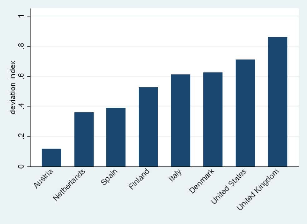
Note: The graph shows the value of the average deviation index at country level, calculated as reported in Equation 1. Source: Authors' calculations based on OECD-ORBIS 2011 and Nesta-FORA firm growth project.
As shown in Figure A1.1 the average deviation index between ORBIS and the NFGD varies from below 0.2 for Austria to above 0.8 for the United Kingdom. The deviation index falls across all countries when considering firms with 10 or more employees, as seen in Figure A1.2, but it is still above 0.25 for most countries. This suggests that comparability of data across different countries for ORBIS to conduct employment dynamics analysis is limited, particularly when smaller firms are included.
Figure A1.2. Average deviation index by country, 2002-2005, firms with 10 employees or more
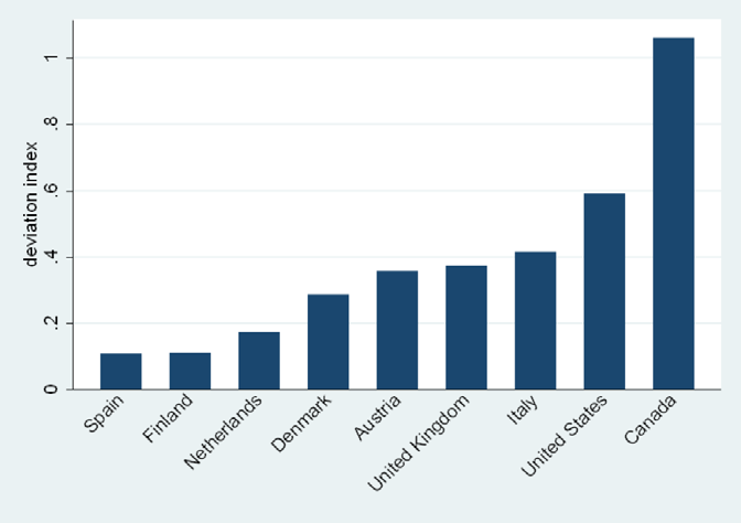
Note: The graph shows the value of the average deviation index at country level, calculated as reported in Equation 1. Source: Authors' calculations based on OECD-ORBIS 2011 and Nesta-FORA firm growth project.
Table A1.11 reports the deviation index across countries in different growth bracket cells. The table highlights all values above 0.25. The table clearly shows large differences between ORBIS and NGFD when all firms with one or more employees are considered. The mean deviation index is above 0.25 for all countries. There are however differences within the distribution. The gap for the share of high-growth firms is relatively smaller for most countries, while the gap for the share of firms growing or shrinking slowly is relatively larger. Figure A1.3 plots the table graphically.
Table A1.11. Deviation index by country, 2002-2005 Growth measured by employment
| [-∞;<-20%[ | [-20%;-15%[ | [-15%;-10%[ | [-10%;-5%[ | [-5%;-1%[ | [-1%;+1%[ | [+1%;+5%[ | [+5%;+10%[ | [+10%;+15%[ | [+15%;+20%[ | [+20%;+∞] | Average | |
|---|---|---|---|---|---|---|---|---|---|---|---|---|
| Austria | 0.02 | 0.39 | 0.08 | 0.15 | 0.03 | 0.02 | 0.17 | 0.03 | 0.19 | 0.19 | 0.04 | 0.12 |
| Canada (firms with 10-249 employees) | 1.40 | 1.20 | 1.23 | 1.14 | 1.52 | 1.44 | 1.35 | 1.07 | 0.50 | 0.56 | 0.27 | 1.06 |
| Denmark | 0.68 | 0.17 | 0.39 | 0.53 | 0.99 | 1.09 | 0.99 | 0.69 | 0.08 | 0.72 | 0.58 | 0.63 |
| Finland | 0.55 | 0.70 | 0.25 | 0.40 | 0.95 | 0.81 | 0.81 | 0.41 | 0.20 | 0.54 | 0.21 | 0.53 |
| Italy | 0.09 | 1.24 | 0.77 | 0.83 | 0.78 | 1.19 | 0.62 | 0.34 | 0.21 | 0.55 | 0.08 | 0.61 |
| Netherlands | 0.42 | 0.18 | 0.19 | 0.22 | 0.73 | 0.38 | 0.79 | 0.28 | 0.51 | 0.01 | 0.28 | 0.36 |
| Spain | 0.29 | 0.40 | 0.17 | 0.44 | 0.71 | 0.35 | 0.71 | 0.53 | 0.15 | 0.43 | 0.13 | 0.39 |
| United Kingdom | 0.43 | 0.79 | 0.47 | 0.95 | 1.44 | 0.92 | 1.48 | 1.23 | 0.58 | 0.97 | 0.24 | 0.86 |
| United States | 1.34 | 0.85 | 1.06 | 0.34 | 0.93 | 0.44 | 1.23 | 0.69 | 0.10 | 0.49 | 0.34 | 0.71 |
Source: Authors' calculations based on OECD-ORBIS 2011 and Nesta-FORA firm growth project.
Table A1.12 examines the deviation index broken down by size. The general pattern that emerges suggests that the accuracy of commercial databases improves with firm size, even if there are some exceptions. However, there are large differences across countries regarding the size threshold above which ORBIS accuracy becomes acceptable (0.25 deviation index). At one extreme, the index for Spain is 0.11 or less for firms that are just above 10 employees. In the middle, for countries like the Netherlands the difference between ORBIS and NFGD only becomes small for firms above 50 employees. At the other extreme, the deviation index is around 0.5 or higher for firms of all sizes in the United States.
Figure A1.3. Average deviation index by growth interval, 2002-2005
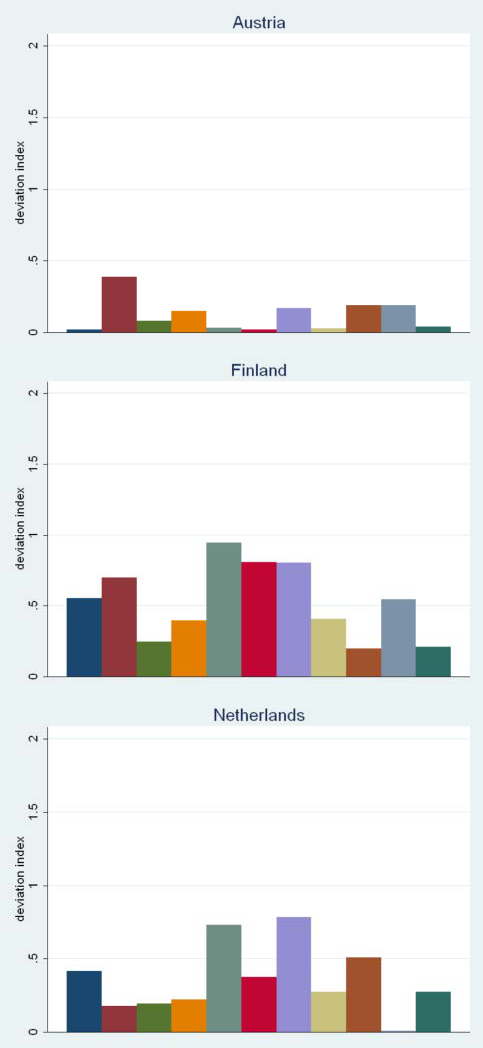
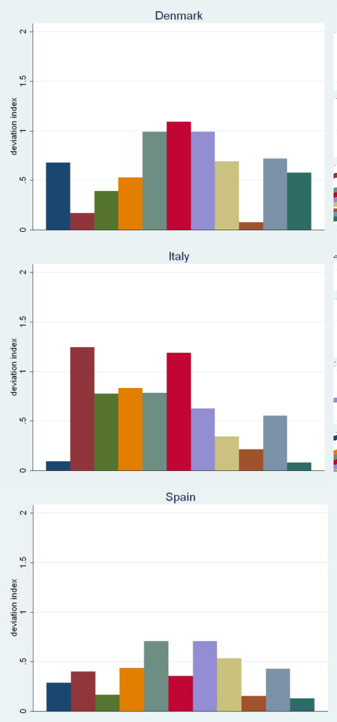
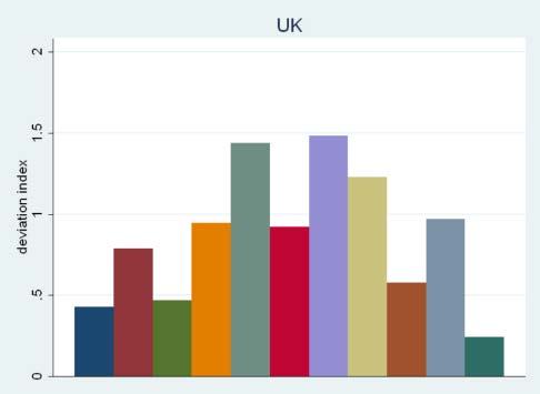
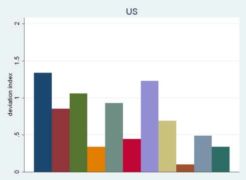
Note: The bars correspond to the deviation index calculated as described in Equation1 in each of the following eleven yearly employment growth interval: [-∞;<-20%[, [-20%;-15%[, [-15%;-10%[, [-10%;-5%[, [-5%;-1%[, [-1%;+1%[, [+1%;+5%[, [+5%;+10%[, [+10%;+15%[, [+15%;+20%[, [+20% ;+∞]. Data for the United Kingdom are preliminary. Source: Authors' calculations based on OECD-ORBIS 2011 and Nesta-FORA firm growth project.
Table A1.13 considers instead the deviation index broken by age. Note that firm growth data broken down by age class was only available for a subset of the countries participating in the Nesta-FORA firm growth project. There is some evidence that the deviation index becomes smaller as firms age, although with quite a few exceptions. Whether this pattern is driven by size (e.g. younger firms being smaller or vice versa) is examined by Figure A1.4, which shows that the deviation decreases with age for micro-firms but not for firms with 10 or more employees.
Table A1.12. Deviation index by country and by firm size class, 2002-2005 Growth measured by employment
| Size class | [-∞;<-20%[ | [-20%;-15%[ | [-15%;-10%[ | [-10%;-5% [ | [-5%;-1%[ | [-1%;+1%[ | [+1%;+5% [ | [+5%;+10%[ | [+10%;+15%[ | [+15%;+20% [[+20%;+∞] | Average | |:----------|----------:|----------:|----------:|----------:|----------:|----------:|----------:|----------:|----------:|----------:|----------:|----------:| | 1-9 employees | 0.19 | 0.26 | 0.09 | 0.10 | 0.30 | 0.05 | 0.06 | 0.07 | 0.12 | 0.42 | 0.26 | 0.17 | | 10-49 employees | 0.32 | 0.14 | 0.12 | 0.14 | 0.54 | 0.94 | 0.66 | 0.44 | 0.13 | 0.33 | 0.12 | 0.35 | | Austria 50-249 employees | 0.87 | 0.70 | 0.40 | 0.21 | 0.32 | 0.67 | 1.06 | 0.36 | 0.50 | 0.37 | 0.42 | 0.54 | | 250+ employees | 1.11 | 0.99 | 0.62 | 0.09 | 0.02 | 0.28 | 0.22 | 1.55 | 0.67 | 2.00 | 1.07 | 0.78 | | 10-49 employees | 1.46 | 1.21 | 1.24 | 1.13 | 1.54 | 1.44 | 1.35 | 1.05 | 0.38 | 0.55 | 0.20 | 1.05 | | Canada 50-249 employees | 1.31 | 1.19 | 1.21 | 1.19 | 1.50 | 1.42 | 1.33 | 1.07 | 1.13 | 0.69 | 0.62 | 1.15 | | 1-9 employees | 0.37 | 2.00 | 2.00 | 1.21 | 2.00 | 0.62 | 0.69 | 0.73 | 0.80 | 0.65 | 0.17 | 1.02 | | 10-49 employees | 1.23 | 0.62 | 1.17 | 0.28 | 0.03 | 0.83 | 0.09 | 0.09 | 0.89 | 0.83 | 0.24 | 0.57 | | Denmark 50-249 employees | 0.16 | 0.15 | 0.83 | 0.48 | 0.14 | 0.18 | 0.02 | 0.41 | 0.40 | 0.35 | 0.82 | 0.36 | | 250+ employees | 2.00 | 2.00 | 0.50 | 0.07 | 0.27 | 0.54 | 0.37 | 0.36 | 0.41 | 0.59 | 0.07 | 0.65 | | 1-9 employees | 0.70 | 1.03 | 0.31 | 0.59 | 1.69 | 0.94 | 1.52 | 0.70 | 0.25 | 0.72 | 0.31 | 0.80 | | 10-49 employees | 0.04 | 0.09 | 0.09 | 0.13 | 0.21 | 0.33 | 0.08 | 0.10 | 0.13 | 0.09 | 0.11 | 0.13 | | Finland 50-249 employees | 0.14 | 0.11 | 0.17 | 0.06 | 0.06 | 0.09 | 0.01 | 0.05 | 0.25 | 0.04 | 0.14 | 0.10 | | 250+ employees | 0.04 | 0.03 | 0.29 | 0.11 | 0.04 | 0.05 | 0.14 | 0.14 | 0.48 | 0.32 | 0.10 | 0.16 | | 1-9 employees | 0.06 | 0.74 | 0.21 | 0.38 | 0.14 | 0.88 | 0.75 | 0.40 | 0.15 | 0.91 | 0.56 | 0.47 | | Italy 10-49 employees | 0.21 | 0.69 | 0.54 | 0.32 | 0.32 | 0.56 | 0.45 | 0.22 | 0.06 | 0.25 | 0.59 | 0.38 | | 50-249 employees | 0.52 | 1.15 | 1.02 | 0.57 | 0.31 | 0.79 | 0.80 | 0.55 | 0.31 | 0.29 | 0.05 | 0.58 | | 250+ employees | 0.75 | 0.84 | 0.65 | 0.44 | 0.26 | 0.59 | 0.60 | 0.15 | 0.19 | 0.20 | 0.56 | 0.48 | | 1-9 employees | 0.17 | 0.57 | 0.56 | 0.45 | 0.80 | 0.08 | 0.33 | 0.33 | 0.51 | 0.19 | 0.51 | 0.41 | | 10-49 employees | 0.23 | 0.40 | 0.57 | 0.26 | 0.23 | 0.47 | 0.05 | 0.03 | 0.01 | 0.25 | 0.79 | 0.30 | | Netherlands 50-249 employees | 0.07 | 0.15 | 0.28 | 0.13 | 0.07 | 0.31 | 0.02 | 0.12 | 0.01 | 0.04 | 0.07 | 0.12 | | 250+ employees | 0.04 | 0.31 | 0.25 | 0.18 | 0.10 | 0.16 | 0.18 | 0.20 | 0.02 | 0.00 | 0.36 | 0.17 | | 1-9 employees | 0.28 | 0.39 | 0.17 | 0.47 | 0.53 | 0.24 | 0.68 | 0.61 | 0.27 | 0.54 | 0.02 | 0.38 | | 10-49 employees | 0.26 | 0.10 | 0.08 | 0.00 | 0.07 | 0.35 | 0.04 | 0.05 | 0.12 | 0.11 | 0.02 | 0.11 | | Spain 50-249 employees | 0.18 | 0.10 | 0.06 | 0.01 | 0.04 | 0.19 | 0.10 | 0.02 | 0.08 | 0.16 | 0.23 | 0.11 | | 250+ employees | 0.17 | 0.05 | 0.02 | 0.04 | 0.06 | 0.05 | 0.06 | 0.01 | 0.02 | 0.15 | 0.07 | 0.06 | | 1-9 employees | 0.34 | 0.73 | 0.54 | 0.94 | 1.26 | 0.26 | 1.26 | 1.09 | 0.63 | 0.96 | 0.03 | 0.73 | | 10-49 employees | 0.50 | 0.11 | 0.06 | 0.18 | 0.40 | 1.02 | 0.62 | 0.52 | 0.50 | 0.49 | 0.35 | 0.43 | | United Kingdom 50-249 employees | 0.77 | 0.36 | 0.25 | 0.05 | 0.26 | 0.34 | 0.42 | 0.33 | 0.25 | 0.04 | 0.31 | 0.31 | | 250+ employees | 0.31 | 0.41 | 0.18 | 0.07 | 0.25 | 0.12 | 0.26 | 0.07 | 0.01 | 0.22 | 0.29 | 0.20 | | 1-9 employees | 1.22 | 0.65 | 0.88 | 0.16 | 1.26 | 0.00 | 1.17 | 0.55 | 0.26 | 0.11 | 0.15 | 0.58 | | 10-49 employees | 1.48 | 1.45 | 1.45 | 0.75 | 0.12 | 0.75 | 0.44 | 0.14 | 0.11 | 0.26 | 0.36 | 0.66 | | United States 50-249 employees | 1.24 | 1.33 | 1.09 | 0.88 | 0.17 | 0.61 | 0.50 | 0.23 | 0.15 | 0.14 | 0.11 | 0.59 | | 250+ employees | 0.71 | 0.49 | 0.60 | 0.34 | 0.33 | 0.08 | 0.16 | 0.43 | 0.61 | 0.73 | 0.72 | 0.47 |
Source: Authors' calculations based on OECD-ORBIS 2011 and Nesta-FORA firm growth project.
Table A1.613. Deviation index by country and by firm age class, 2002-2005 Growth measured by employment
| Age class | [-∞;<-20%[ | [-20%;-15%[ | [-15%;-10% [ | [-10%;-5% [[-5%;-1%[ | [-1%;+1% [ | [+1%;+5% [[+5%;+10%[ | [+10%;+15% [ | [+15%;+20%[ | [+20%;+∞] | Average | |:----------|----------:|----------:|----------:|----------:|----------:|----------:|----------:|----------:|----------:|----------:|----------:|----------:| | 1-5 years | 0.26 | 0.41 | 0.23 | 0.18 | 0.33 | 0.00 | 0.24 | 0.09 | 0.29 | 0.00 | 0.18 | 0.20 | | Austria 6-10 years | 0.06 | 0.13 | 0.09 | 0.12 | 0.27 | 0.02 | 0.07 | 0.08 | 0.23 | 0.31 | 0.22 | 0.14 | | 11+ years | 0.11 | 0.41 | 0.17 | 0.07 | 0.08 | 0.02 | 0.37 | 0.06 | 0.08 | 0.31 | 0.09 | 0.16 | | 1-5 years | 0.76 | 2.00 | 0.68 | 1.07 | 1.28 | 0.91 | 0.72 | 0.76 | 0.48 | 0.32 | 0.76 | 0.89 | | Denmark 6-10 years | 0.78 | 2.00 | 0.13 | 0.78 | 0.70 | 0.69 | 0.57 | 0.17 | 0.34 | 1.09 | 0.33 | 0.69 | | 11+ years | 0.37 | 0.70 | 0.33 | 0.31 | 1.02 | 1.25 | 0.85 | 0.69 | 0.37 | 0.73 | 0.24 | 0.62 | | 1-5 years | 0.66 | 0.82 | 0.14 | 0.50 | 1.15 | 0.84 | 1.04 | 0.63 | 0.21 | 0.54 | 0.10 | 0.60 | | Finland 6-10 years | 0.60 | 0.79 | 0.32 | 0.52 | 1.12 | 0.91 | 1.01 | 0.52 | 0.15 | 0.67 | 0.28 | 0.63 | | 11+ years | 0.48 | 0.61 | 0.26 | 0.33 | 0.84 | 0.73 | 0.67 | 0.27 | 0.24 | 0.40 | 0.38 | 0.47 | | 1-5 years | 0.03 | 1.05 | 0.60 | 0.64 | 0.74 | 1.10 | 0.72 | 0.34 | 0.15 | 0.62 | 0.19 | 0.56 | | Italy 6-10 years | 0.06 | 1.06 | 0.53 | 0.70 | 0.85 | 1.14 | 0.73 | 0.43 | 0.10 | 0.72 | 0.14 | 0.59 | | 11+ years | 0.15 | 1.29 | 0.82 | 0.83 | 0.70 | 1.24 | 0.52 | 0.28 | 0.25 | 0.54 | 0.13 | 0.61 | | 1-5 years | 0.40 | 0.14 | 0.12 | 0.26 | 0.91 | 0.30 | 0.59 | 0.48 | 0.24 | 0.04 | 0.06 | 0.32 | | Netherlands 6-10 years | 0.21 | 0.30 | 0.29 | 0.13 | 0.97 | 0.46 | 0.86 | 0.15 | 0.55 | 0.25 | 0.15 | 0.39 | | 11+ years | 0.43 | 0.19 | 0.26 | 0.11 | 0.53 | 0.35 | 0.66 | 0.20 | 0.51 | 0.06 | 0.14 | 0.31 |
Source: Authors' calculations based on OECD-ORBIS 2011 and Nesta-FORA firm growth project.
Figure A1.4. Average deviation index by firm size and age, 2002-2005
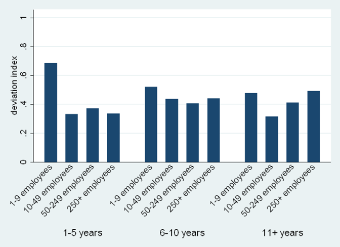
Note: The graph shows the value of the average deviation index calculated as reported in Equation 1. Firms are classified in 12 groups based on the combination of 3 age classes (1-5, 6-10, 11+) and 4 size classes (1-9, 10-49, 50-249, 250+). Source: Authors' calculations based on OECD-ORBIS 2011 and Nesta-FORA firm growth project.
Figure A1.5 Average deviation index by sector, 2002-2005
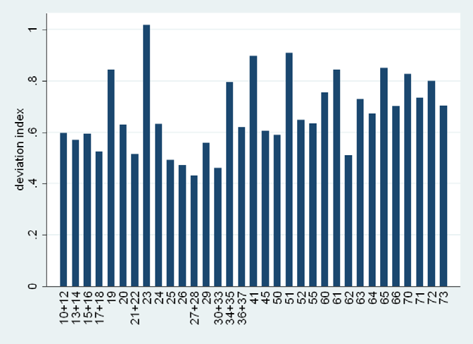
Note: The graph shows the value of the average deviation index at industry level, calculated as reported in Equation 1. Source: Authors' calculations based on OECD-ORBIS 2011 and Nesta-FORA firm growth project.
Figure A1.5 examines the deviation index by sector. For simplicity, the index is aggregated across all countries (the underlying tables showing the deviation index by sector for each country are available upon request). While no clear pattern emerges, the data appears to suggest that the deviation index is generally larger for services sectors than for manufacturing. Manufacturing has the sector with the lowest deviation index (27+28: Basic metals and fabricated metal products) but also one of the highest (23: Coke, refined petroleum products and nuclear fuel). Figure A1.6 shows the same graph restricted to firms with 10 employees or more. In general deviations are lower, and manufacturing and services sector look now more similar in values. However, there is still a large variability across sectors, both within manufacturing and services.
Figures A1.7, A1.8, A1.9, A1.10 and A1.11 below undertake the same analysis but considering instead the second period for which the NFGD is available (2004-2007). In a nutshell, the same patterns emerge. Despite the progressive increase in coverage in ORBIS over the decade, the results do not yet show that there has been a marked decrease in the deviation index from the first to the second period.
Figure A1.6. Average deviation index by sector, 2002-2005, firms with 10 employees or more
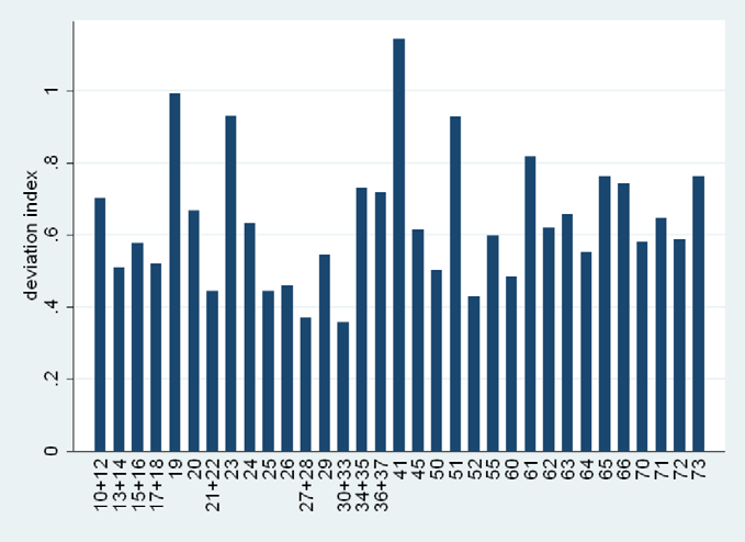
Note: The graph shows the value of the average deviation index at industry level, calculated as reported in Equation 1. Source: Authors' calculations based on OECD-ORBIS 2011 and Nesta-FORA firm growth project.
Figure A1.7. Average deviation index by country, 2004-2007, all firms
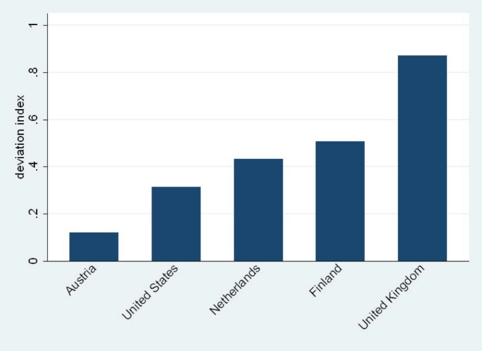
Note: The graph shows the value of the average deviation index at country level, calculated as reported in Equation 1. Source: Authors' calculations based on OECD-ORBIS 2011 and Nesta-FORA firm growth project.
Figure A1.8. Average deviation index by country, 2004-2007, firms with 10 or more employees
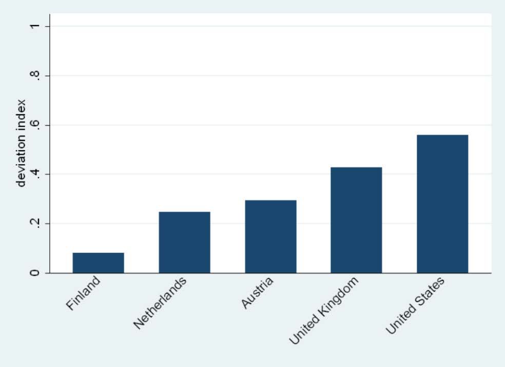
Note: The graph shows the value of the average deviation index at country level, calculated as reported in Equation 1. Source: Authors' calculations based on OECD-ORBIS 2011 and Nesta-FORA firm growth project.
Figure A1.9. Average deviation index by sector, 2004-2007
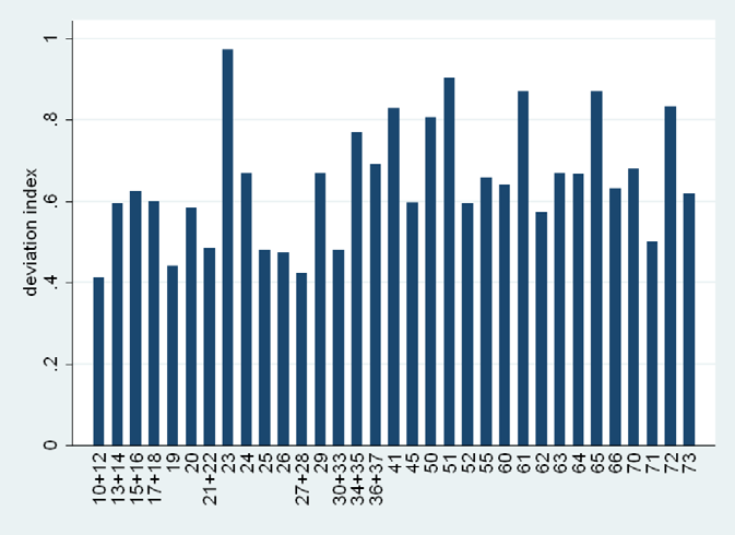
Note: The graph shows the value of the average deviation index at industry level, calculated as reported in Equation 1. Source: Authors' calculations based on OECD-ORBIS 2011 and Nesta-FORA firm growth project.
Figure A1.10. Average deviation index by size and age, 2004-2007
Note: The graph shows the value of the average deviation index calculated as reported in Equation 1. Firms are classified in 12 groups based on the combination of 3 age classes (1-5, 6-10, 11+) and 4 size classes (1-9, 10-49, 50-249, 250+). Source: Authors' calculations based on OECD-ORBIS 2011 and Nesta-FORA firm growth project.
Figure A1.11. Average deviation index by growth interval, 2004-2007
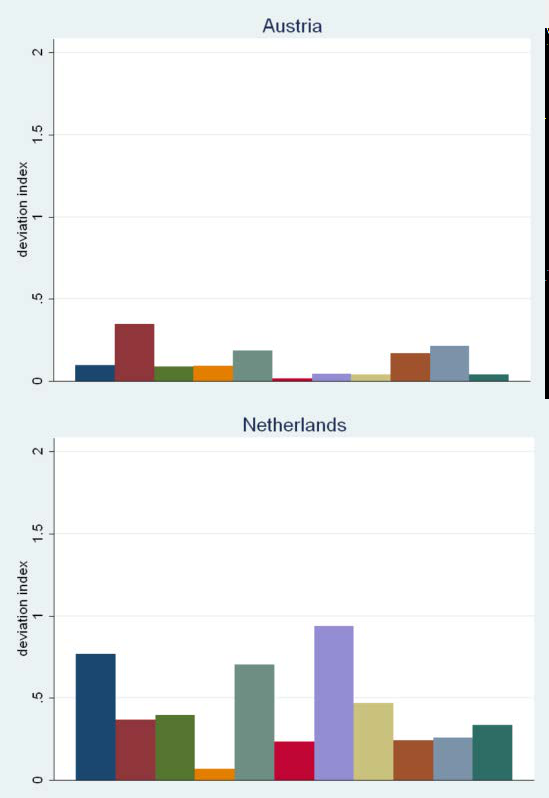
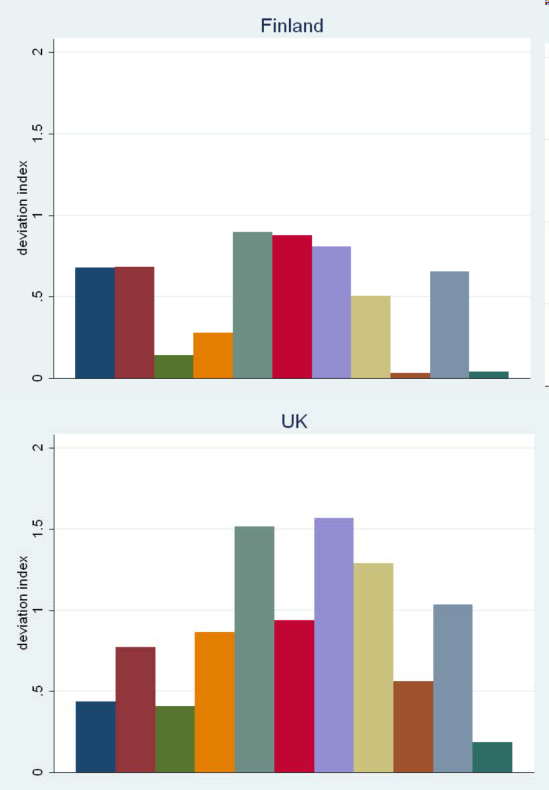
III. Concluding remarks
The analysis in this appendix exposes important differences between data derived from business registers and commercial databases. There are large (and heterogeneous) differences in the coverage of firms included in OECD-ORBIS 2011 relative to the database collected by FORA and Nesta. Moreover, the analysis suggests that the differences go beyond the level of coverage and have a significant impact on the growth indicators derived from them. The expansion in the coverage of ORBIS in the past few years may help to mitigate some of these differences. However, while ORBIS constitutes an extremely valuable resource for research, the results highlight the importance of continuing to undertake harmonised micro-aggregated data collection using official business registers, building on the work pioneered by the OECD a decade ago (Bartelsman et al. 2004).
-
Data for Canada are not available at a detailed sectoral level. Therefore Canada is not included in the regression analysis and any other analysis requiring industry breakdowns. The United States is also excluded from the econometric analysis since it is used as the benchmark economy. ↩
-
www.oecd.org/document/58/0,3343,en_2649_44392116_44441658_1_1_1_1,00.html ↩
-
Specifically, the 11 growth intervals considered are: ]-∞,-20%[, [-20%;-15%[, [-15%;-10%[, [-10%;-5%[, [-5%;-1%[, [-1%;1%[, [1%;5%[, [5%;10%[, [10%;15%[, [15%;20%[ and [20%;∞[. ↩
-
See Bravo-Biosca (2010b) for details on the approach followed to do so. ↩
-
These concerns are more significant for the largest firms, for which consolidated statements provided by commercial databases are a useful resource. See Hoffman and Junge (2006) for further discussion. ↩
-
The discussion in this section uses the data for ten countries (data for Greece was added later and it is not included here), while the regression analysis in the section that follows considers only nine countries for which sufficient industry detail was available. ↩
-
Decreasing, stable, growing and high-growth firms are defined according to the following growth rate intervals, respectively: [-∞;-5%[, [-5%;+5%[, [+5%;+20%[, [+20%;+∞]. Unless otherwise stated, all growth rate data refers to firms with 10 employees or more. ↩
-
The graph plots the residuals from an OLS regression of the two variables on industry and country fixed effects. ↩
-
Sectoral level figures (reported in Appendix B for brevity) show that all manufacturing sectors are shrinking, while the majority of service sectors are growing. Going down to the specific manufacturing sectors: textiles (ISIC 17-18) and leather and footwear (ISIC 19) went through sharp contractions in employment, but a few other manufacturing sectors showed a positive trend (wood and furniture, coke and petroleum, rubber, non-metallic products, basic and fabricated metals). ↩
-
See table notes for details. ↩
-
Note that the ranking of industries is taken from the benchmark country, i.e. the United States and the level of R&D intensity in different industries is provided in Table A.2 in Appendix A. Similarly, the strictness of EPL in different countries is provided in Table A.1 in Appendix A. ↩
-
Note that the ranking of industries is taken from the benchmark country, i.e. the United States, and the level of R&D intensity in different industries can be found in Table A.2 in Appendix A. Similarly, the tightness of EPL in different countries can be found in Table A.1 in Appendix A. ↩
-
The analysis on the role of private bankruptcy regimes is available from the authors upon request. ↩
-
The measure includes interest paid and fees, but excludes loans. Therefore, it serves as a proxy for dependence on external finance but more broadly it captures the industries that consume more financial services (and are therefore likely to benefit the most from a developed financial market). It is not possible to use the external finance dependence measure originally developed by Rajan and Zingales (1998) since this was based on the external finance needs of US listed companies obtained from Compustat. The instrumental variables approach used here requires information on external finance needs in all the countries in the sample. However, in most of them the stock market plays a smaller role than in the United States and it is likely to be less representative of the external finance needs of a particular industry in the country, while the available data on external finance dependence for non-listed companies is much more limited. Excluding the financial sector from this analysis leads to very similar results. ↩
-
The relative generosity of R&D tax provisions has been calculated for large and small firms using as indicator one minus the B-index (Warda, 2001). The value of the B-index is based on the before-tax income required to break even on one dollar of R&D outlays and takes into account corporate income tax rates, R&D tax credits, special R&D allowances from taxable income, and depreciation of capital assets (machinery, equipment and buildings) used in R&D so that it becomes profitable to perform research activities. ↩
-
We thankfully acknowledge research assistance by Elif Köksal-Oudot for the analysis conducted in this Appendix. ↩
-
The name, as well as all the content of the ORBIS database, is protected by copyrights of Bureau van Dijk Electronic Publishing (BvDEP). In the following, the sign is dropped in order to ease readability. ↩
-
This discussion draws extensively on Bravo-Biosca (2010b). ↩
-
Data for Greece was added more recently to the database and it is not included in this discussion. ↩
-
Specifically, the 11 growth intervals considered are: ]-∞,-20%[, [-20%;-15%[, [-15%;-10%[, [10%;-5%[, [-5%;-1%[, [-1%;1%[, [1%;5%[, [5%;10%[, [10%;15%[, [15%;20%[ and [20%;∞[. ↩
-
The failure to record multinational expansion may have a different impact depending on the size of the country. If a firm opens a new plant 1000 miles away from its headquarters, it is likely measured as growth in the US but most likely not in the Netherlands, since this plant would be based in a different country. ↩
-
These concerns are more significant for the largest firms, for which consolidated statements provided by commercial databases are a useful resource. See Hoffmann and Junge (2006) for further discussion. ↩
-
Other countries (1) and Other countries (2) present the number of records by year for higher than 50,000 firms. Other countries (3) presents the number of records by year for less than 50,000 firms. ↩
-
The ORBIS data presented in the tables refer to the OECD-ORBIS 2011 database. ↩
-
Note however that the number of US companies in ORBIS has increased dramatically over the past few years. ↩↩