Alex Coad
SPRU, University of Sussex & Aalborg University, Denmark
Marc Cowling
University of Exeter
Josh Siepel
SPRU, University of Sussex & Aalborg University, Denmark
Nesta Working Paper 12/10
October 2012
www.nesta.org.uk/wp12-10
Abstract
We seek to complement existing research on High-Growth Firms (HGFs) by applying relatively advanced econometric techniques to the analysis of HGF growth processes. Structural Vector Autoregressions (SVARs) show that the growth processes of firms start with employment growth, then sales growth, then assets growth, then profits growth, while the growth processes of HGFs put more emphasis on sales growth driving the other dimensions. We then investigate the possibility of interdependence or 'spillovers' between the growth of HGFs and non-HGFs. Peer-effects econometrics dispel concerns that HGFs should be seen as 'cannibals' that exploit growth opportunities that would otherwise be exploited by other firms.
JEL Classification: L25
Keywords: High growth firms, growth process, SVAR, rivalry, firm growth
We are very much indebted to Albert Bravo Biosca, Louise Marston and Alessio Moneta for many helpful comments, and participants at Nesta workshops for many helpful comments and discussions. Any remaining errors are ours alone. Corresponding Author: Alex Coad, Freeman Centre, SPRU, University of Sussex, Falmer, Brighton, BN1 9QE, UK. [email protected]
The Nesta Working Paper Series is intended to make available early results of research undertaken or supported by Nesta and its partners in order to elicit comments and suggestions for revisions and to encourage discussion and further debate prior to publication (ISSN 2050-9820). © 2012 by the authors. Short sections of text, tables and figures may be reproduced without explicit permission provided that full credit is given to the source. The views expressed in this working paper are those of the author(s) and do not necessarily represent those of Nesta.
1. Introduction
Interest in high-growth firms (HGFs) has exploded in recent years, once the job-creating prowess of a minority of fast-growing firms became recognized – roughly 4% of firms can be expected to generate 50% of jobs (Storey, 1994, p. 117). Research into high-growth firms has itself undergone high-growth. However, the level of analysis has often remained rather simplistic, focusing on either the relative numbers of high-growth firms across countries, or the sectors in which HGFs are relatively abundant, or the determinants and characteristics of HGFs in contradistinction to non-HGFs considering variables such as size and age (Henrekson and Johansson, 2010). Previous work has typically found it extremely hard to predict which firms will become HGFs, and has observed that high-growth episodes are not persistent (a HGF in one year need not be a HGF in the next). HGFs are found in all sectors, especially the services sector (but they are not over-represented in high-tech sectors if anything, they are under-represented here (Henrekson and Johansson, 2010; Mason and Brown, 2010)). Henrekson and Johansson (2010, p. 227) also observe that “it is young age more than small size that is associated with rapid growth." More generally, however, it is difficult to predict which firms will be HGFs. In this paper, we do not seek to predict who will become a HGF. Instead, we seek to complement existing work by applying advanced econometric techniques to get new insights into the processes of high-growth firms.
First, we investigate how growth processes of HGFs unfold, by applying data-driven techniques based on Independent Component Analysis (ICA) for establishing causality, that exploit the non-Gaussian structure of residuals to infer causal relationships. In particular, we build upon the LiNGAM model (Linear Non-Gaussian Acyclic Model) introduced in a cross-sectional context by Shimizu et al. (2006), and extended to a SVAR (Structural Vector Autoregression) context, by introducing lagged effects, by Moneta et al. (2012). This VAR-LiNGAM approach to obtaining causal estimates from observational data is often applied in the neuroimaging literature, although it has recently been introduced into the econometrics literature by Moneta et al. (2012).
Second, we investigate whether HGFs are seen as rivals or sources of beneficial 'spillovers' by other firms in the same industry, by applying peer-effects econometrics. On the one hand, it could be that HGFs rush in to take advantage of economic opportunities by spoiling these opportunities for others, and stealing the market in a 'cannibalistic' sense, in such a hasty way that these opportunities are exploited rather inefficiently. On the other hand, it could be that HGFs play a more complementary role, spotting opportunities that would otherwise remain undeveloped, and generating a number of spillovers (such as knowledge spillovers, productivity spillovers (‘red queen effects'), boosting economic growth through new wealth and new demand, etc) that benefit other firms. Theory is not clear, and so this issue needs to be addressed with empirical evidence.
The structure of the paper is the following. The next section briefly summarizes the relevant literature. Section 2 gives an introduction to firm growth processes in the UK by presenting some simple vector autoregression results based on official ONS data. Section 3 presents the FAME database that will be the focus of our subsequent analysis. In Section 4 we apply some SVAR models to analyze firm growth, first presenting our econometric methodology and then discussing the results. In Section 5 we apply peer-effects econometrics to investigate whether HGFs can be seen as rivals or whether they play a complementary role with regards to other firms. The final section (Section 6) contains our conclusions, where we discuss policy implications of our results.
2. Preliminary findings
To begin with, we present some simple vector autoregression models on firm growth processes, using the available data on sales growth and employment growth, from Office of National Statistics (ONS) data, using the Business Structure Database (BSD) files (for more information on the BSD, see Evans and Welpton (2009)). BSD provides a detailed record of the performance of UK firms, using VAT figures collected by HM Treasury and employment records from National Insurance. Growth rates of sales and employment are calculated by taking log-differences of total sales and total employment. Table 1 looks at vector autoregression models with either 2 or 3 lags. To begin with, we see plenty of evidence of negative autocorrelation in the time series of Sales growth and Employment growth. This negative autocorrelation means that, ceteris paribus, Sales (Employment) growth in any one year is not likely to be followed by Sales (Employment) growth in the following year.
Another interesting result concerns the relationship between size and growth – a relationship often referred to as ‘Gibrat's Law'. We proxy size by taking the lagged natural logarithm of the number of employees. With respect to sales growth, we see that lagged size has a small positive association with subsequent sales growth. With respect to employment growth, however, a larger size is associated with slower growth – and the effect is much larger than for sales growth. Taken together, the evidence suggests that firms with many employees are less likely than their smaller counterparts to experience subsequent employment growth, and that instead they can benefit from growth in a different dimension – sales growth.
With these vector autoregression models, however, we are primarily interested in the interplay of sales and employment growth. The results in Table 1 show that lagged employment helps predict sales growth, and lagged sales growth helps predict subsequent employment growth. Although the results are statistically significant (no doubt bolstered by the large number of observations), the magnitudes of the effects are not especially high. Moreover, the R² statistic remains low, indicating that most of the variation in growth rates remains unexplained. The low R² of growth rate regressions has been observed in many other studies and has been taken as evidence that firm growth is essentially a ‘random walk' process. Looking at the coefficient magnitudes, it appears that lagged employment growth has a slightly larger contribution to subsequent sales growth than vice versa (lagged sales growth on subsequent employment growth), because the respective coefficients are 0.13-0.14 versus 0.05-0.06 at the first lag. The magnitude of the effects fades as the number of lags increases.
Table 2 presents the results of a size disaggregation exercise. These results show that, for smaller firms, employment growth plays a more important role with regards to subsequent sales growth, although there are also significant effects of sales growth on subsequent employment growth. As our focus shifts towards larger firms (250+ employees), the co-evolutionary link between sales growth and employment growth becomes weaker.
Sales growth and employment growth appear to be more 'mutually reinforcing' in the case of smaller firms. The growth of small firms is qualitatively different from the growth of larger firms – smaller firms must struggle through the 'liability of newness' to achieve economies of scale, and the ‘grow or die' dilemma is especially acute for these firms. Smaller firms also enjoy a more flexible organizational structure, and so can respond better to new human resources to put them to work on new tasks in imaginative ways. For larger firms, in constrast, sales and employment growth appear to be more random and less inter-related, perhaps because selection pressures are less severe for these established firms who have reached the ‘minimum efficient scale' (MES).
Table 2 also contains evidence on the relationship between size and growth. The coefficients on lagged size in Table 2 indicate that larger firms tend to experience slower growth in terms of both sales and employment – a finding often referred to as Galtonian ‘reversion to the mean'. This negative dependence of growth on size has been observed in previous empirical literature (see for example Sutton, 1997; Caves, 1998; Coad, 2009). While small firms must struggle to grow to overcome their size disadvantage, larger firms that have achieved a minimum efficient scale are under less pressure to grow.
Table 3 looks specifically at the growth processes of the firms that are growing fastest in terms of sales or employment. For the subsample of Sales HGFs, we see that sales growth has a slightly larger association with subsequent employment growth than in the case of Employment HGFs. For the subsample of Employment HGFs, we see that employment has a considerably larger association with subsequent sales growth than in the case of Sales HGFs. In other words, firms with the 5% fastest employment growth are seen to efficiently ‘convert' this employment growth into sales growth – in the sense that employment growth in these firms makes an especially visible impact on subsequent sales growth. These firms appear to be more capable of internalizing new human resources to fuel subsequent growth of sales.
These results can be broadly interpreted as follows: employment growth and sales growth are two related but distinct dimensions of firm size and growth. To be sure, large firms are large in terms of both sales and employment, but during their growth there may well be stages in the growth of sales and employment where one variable has a larger impact on the other, where one leads and the other follows. We would like to know the causal ordering of these firm growth variables – not just intertemporal associations from one year to the next, but ideally see how sales growth and employment growth affect each other in the shorter term – within the same period. If we focus only on lags of one year or more (in the context of reduced-form vector autoregressions) then we might miss out on some important within-the-period effects that fade out in the longer-term. To get a better understanding of the processes of firm growth, we need to peer inside the 'black box' of instantaneous causal effects – how sales growth and employment growth (and perhaps other facets of firm growth not covered in the ONS ABS data) causally affect each other within the same year, also considering lagged effects.
|
Sales gr. |
t-stat |
Empl gr. |
t-stat |
Sales gr. |
t-stat |
Empl gr. |
t-stat |
|
2 lags |
|
|
|
3 lags |
|
|
|
| Sales gr. (lagged) |
-0.18539 |
-100.84 |
0.060222 |
114.03 |
-0.20055 |
-86.3 |
0.052872 |
87.8 |
| Empl gr. (lagged) |
0.141156 |
92.94 |
-0.03012 |
-29.12 |
0.1265 |
75.14 |
-0.03511 |
-31.85 |
| Sales gr. (2nd lag) |
-0.06156 |
-41.52 |
0.034319 |
77.09 |
-0.07271 |
-35.48 |
0.039726 |
75.04 |
| Empl gr. (2nd lag) |
0.061671 |
44.64 |
-0.02492 |
-27.9 |
0.058675 |
36.76 |
-0.02892 |
-29.41 |
| Sales gr. (2nd lag) |
|
|
|
|
-0.02967 |
-17.76 |
0.03014 |
62.14 |
| Empl gr. (2nd lag) |
|
|
|
|
0.041346 |
25.87 |
-0.01561 |
-16.25 |
| Sales/Empl |
8.78E-05 |
8.03 |
-9.27E-06 |
-6.70 |
0.000123 |
5.88 |
-1.5E-05 |
-5.47 |
| (Sales/Empl)² |
-1.30E-10 |
-4.68 |
1.38E-11 |
4.14 |
-1.60E-10 |
-6.21 |
1.93E-11 |
5.76 |
| log(Empl), lagged |
0.00449 |
10.78 |
-0.03921 |
-136.54 |
0.005476 |
11.54 |
-0.02941 |
-89.7 |
| Constant |
0.007931 |
5.94 |
0.08305 |
148.28 |
-0.004 |
-1.80 |
0.056948 |
85.79 |
| Observations |
3014995 |
|
3014995 |
|
2245566 |
|
2245566 |
|
| R² |
0.0399 |
|
0.0242 |
|
0.0468 |
|
0.0231 |
|
Table 1: Vector autoregression models on ONS/ABS data for sales and employment growth, for VAR models including either 2 or 3 lags. Coefficients and t-statistics.
3. Database
For our advanced econometric analysis, which requires a relatively large number of variables as well as recent developments in econometric theory and software, we use data on UK businesses from FAME (Financial Analysis Made Easy). FAME data has some advantages over Census data in that it provides information on a number of variables – not just sales and employment, but also other variables such as financial performance and growth of assets. We take growth of operating surplus as an indicator of the financial performance of the firm, which we consider to be a better indicator than net profit, although we are aware that financial performance variables can sometimes be unreliable proxies for the underlying economic phenomena of interest (Fisher and McGowan, 1983), and therefore should be treated with some caution. For a more detailed comparison of the BSD and FAME datasets, and why we use both in this analysis, see Appendix A.
Turnover, Net Tangible Assets and Operating Profit are defined in terms of thousands of GBP, and for number of employees we take the headcount of employees. With regards to identifying industrial sectors, we use 2007 SIC Codes, and recode them at the level of 3-digit, 4-digit or 5-digit industries. We focus on the years 2003-2011, although many of the firms included in our analysis do not report data for the full period (that is, we have an unbalanced panel).
|
|
Sales gr. |
t-stat |
Empl gr. |
t-stat |
Sales gr. |
t-stat |
Empl gr. |
t-stat |
Sales gr. |
t-stat |
Empl gr. |
t-stat |
|
|
10+ employees |
|
|
|
50+ employees |
|
|
|
250+ employees |
|
|
|
| Sales gr. (lagged) |
|
-0.16097 |
-46.29 |
0.06593 |
47.2 |
-0.20769 |
-17.45 |
0.031657 |
5.24 |
-0.28058 |
-4.35 |
-0.00038 |
-0.01 |
| Empl gr. (lagged) |
|
0.04842 |
55.38 |
0.023006 |
11.43 |
0.122227 |
11.51 |
-0.02496 |
-2.55 |
0.021806 |
0.39 |
-0.20816 |
-4.20 |
| Sales gr. (second lag) |
|
-0.05246 |
-20.05 |
0.049579 |
43.96 |
-0.08565 |
-9.28 |
0.036654 |
7.86 |
-0.16782 |
-3.68 |
-0.01765 |
-0.61 |
| Empl gr. (second lag) |
|
0.075645 |
31.74 |
0.004272 |
2.47 |
0.084922 |
9.54 |
-0.00427 |
-0.58 |
0.069145 |
1.37 |
-0.04864 |
-1.37 |
| Sales/Empl |
|
0.000183 |
7.99 |
-4.2E-05 |
-6.90 |
0.000203 |
9.03 |
-0.0001 |
-4.05 |
0.000317 |
1.86 |
-0.00038 |
-2.43 |
| (Sales/Empl)² |
|
-7.03E-10 |
-5.33 |
1.70E-10 |
5.89 |
-5.91E-10 |
-8.04 |
3.39E-10 |
4.04 |
-2.87E-08 |
-1.96 |
8.69E-09 |
0.47 |
| log(Empl), lagged |
|
-0.02626 |
-23.25 |
-0.12122 |
-119.77 |
-0.07177 |
-14.00 |
-0.17949 |
-31.74 |
-0.10826 |
-5.62 |
-0.15594 |
-8.91 |
| Constant term |
|
0.105887 |
23.87 |
0.380819 |
123.52 |
0.385226 |
17.24 |
0.834986 |
33.57 |
0.819693 |
5.66 |
1.162584 |
8.89 |
| Observations |
|
820770 |
|
820770 |
|
60374 |
|
60374 |
|
2095 |
|
2095 |
|
| R² |
|
0.0401 |
|
0.0661 |
|
0.0577 |
|
0.1048 |
|
0.1225 |
|
0.1422 |
|
Table 2: Vector autoregression models on ONS/ABS data for sales and employment growth, for three groups of firms (mean size of 10+, 50+ and 250+ employees respectively). Coefficients and t-statistics.
In line with previous work, we focus on firms with 20 employees or more.
|
Sales gr. |
t-stat |
Empl gr. |
t-stat |
Sales gr. |
t-stat |
Empl gr. |
t-stat |
|
HGFs: 5% fastest sales growth |
|
|
|
HGFs: 5% fastest empl. growth |
|
|
|
| Sales gr. (lagged) |
-0.30506 |
-64.21 |
0.061278 |
38.65 |
-0.26626 |
-34.59 |
0.046244 |
15.17 |
| Empl gr. (lagged) |
0.040351 |
4.38 |
-0.0761 |
-6.84 |
0.213195 |
20.21 |
-0.15564 |
-19.65 |
| Sales gr. (second lag) |
-0.19412 |
-39.41 |
0.043284 |
28.03 |
-0.09591 |
-16.25 |
0.034386 |
13.24 |
| Empl gr. (second lag) |
0.062832 |
7.34 |
-0.06156 |
-7.22 |
0.07987 |
9.61 |
-0.12376 |
-19.92 |
| Sales/Empl |
0.000127 |
10.05 |
-3.2E-05 |
-8.47 |
0.00024 |
7.55 |
-5.38E-06 |
-1.15 |
| (Sales/Empl)² |
-4.42E-10 |
-4.42 |
1.25E-10 |
5.10 |
-1.26E-09 |
-6.19 |
2.59E-11 |
1.08 |
| log(Empl), lagged |
0.053245 |
17.30 |
-0.01825 |
-7.49 |
0.065122 |
23.72 |
0.008354 |
4.35 |
| Constant term |
1.037868 |
151.09 |
0.183865 |
40.57 |
0.078607 |
14.08 |
0.677102 |
198.89 |
| Observations |
113769 |
|
113769 |
|
163424 |
|
163424 |
|
| R² |
0.1605 |
|
0.0275 |
|
0.0808 |
|
0.0203 |
|
Table 3: Vector autoregression models on ONS/ABS data for sales and employment growth, for subsamples of High-Growth Firms (measured as 5% fastest growing firms in terms of sales or employment, respectively). Coefficients and t-statistics.
smaller firms would amplify difficulties of missing observations and hence selection bias. Instead, we focus on firms with 20 employees or more, and so our results should be interpreted accordingly. Therefore our analysis does not include the smallest firms in the economy, with fewer than 20 employees.
In our subsequent analysis, we sometimes split the sample into subsamples of HGFs versus non-HGFs. This is done in the following way: first we calculate a firm's average annual employment growth over the available time period (with a minimum of at least 3 years). If we consider that a firm's average annual employment growth rate $\gamma$ can be expressed in terms of the relationship between initial size $S_t$ and final size $S_{t+\tau}$:
$$
(1 + \gamma)^{\tau} = \frac{S_{t+\tau}}{S_t} \quad \text{(1)}
$$
then the average annual growth rate $\gamma$ can be calculated in the following way:
$$
\left(\frac{S_{t+\tau}}{S_t}\right)^{\frac{1}{\tau}} - 1 = \gamma \quad \text{(2)}
$$
HGFs are then defined as those firms that are in the top 10% of the (average annual) growth rates distribution.
We choose this measure of HGFs in order to exploit the available data as best we can, by making use of all available years (maximum duration: 2003-2011). Firms in our sample are present for different lengths of time, and so we normalize by calculating the average annual growth rate (with a minimum of three years). It has been observed that high-growth events display little persistence (Coad, 2007a; Parker et al., 2010), and therefore we do not focus on what happens after a high-growth event, but only how firms grow during their high-growth period. Although some sectors may grow faster than others, we do not normalize by sector, because we argue that a high employment growth rate is equally challenging (from an organizational point of view) whatever sector the firm operates in. We prefer relative growth to absolute growth, because the latter emphasizes the growth of large firms to the detriment of the growth of smaller firms (Hölzl, 2011). We also focus on the top 10% of the employment growth rates distribution to ensure that we have enough firms in the HGF category, while ensuring that we include as HGFs only those firms that are genuine fast growers.
In our SVAR analysis in Section 4.1.3, we include all firms, whereas in our peer-effects estimates in Section 5 we focus only on larger firms (with a mean size of either 200+, 250+ or 300+ employees), because we consider that larger firms are more likely to be engaged in direct competition whereas small firms can escape direct competition by specializing in niche markets or regions.
4. SVAR models of firm growth
In this section, we seek to unravel the processes of firm growth by considering different facets of the growth process: sales growth, employment growth, growth of assets, and growth of profit margins. We therefore contribute to the literature that considers how firms grow in terms of sales and profits (Cowling, 2004). To this end, we apply Structural Vector Autoregressions (SVARs) – to be precise, we apply a Linear non-Gaussian Acyclic SVAR model (VAR-LiNGAM) that is identified through Independent Component Analysis (ICA). We being by presenting our methodology in non-technical terms before applying it to our FAME data (Section 4.1). Technical details on our methodology, the intuition behind ICA, our identification strategy, and the assumptions on which the estimator is built are presented in Appendix B.
Our reduced-form VAR models presented earlier in Section 2 were interesting in describing the intertemporal associations between two dimensions of firm growth – sales and employment. Although intertemporal associations can describe the evolution of firms over time, they do not identify which variable is driving the other. Correlation does not imply causality – or in everyday language ‘you can't get an ‘ought' from an 'is." Knowledge of the causal relations (as opposed to mere associations) is essential as soon as one wishes to consider how to intervene in the system being observed. A well-placed intervention will target one particular variable to have predictable effects on other variables as the ‘shock' propagates throughout the system. However, without knowledge of the causal relations, a misplaced intervention might have no effect (or even perverse effects) if the variable targeted has no causal effect (or unexpected effects) on the other variables.
One analogy relates to sailing – we observe a boat that is sailing due west, although
|
Sales gr. |
Empl. gr. |
Tot. Ass. gr. |
Op. Prof. gr. |
| Sales gr. |
1 |
|
|
|
| Empl. gr. |
0.5325 |
1 |
|
|
| Tot. Ass. gr. |
0.1954 |
0.1247 |
1 |
|
| Op. Prof. gr. |
0.3412 |
0.1224 |
0.1739 |
1 |
Table 4: Matrix of correlation coefficients for the VAR series. 150'920 observations. All correlations are statistically significantly different from zero at the 5% level.
the rudder is pointing northwest to take into account a wind that blows south. If the rudder was aimed due west (in the desired direction of motion), the boat would not end up in the desired location because of the wind. Simply observing intertemporal dynamics does not provide enough information on which to base an intervention. Instead, knowledge of the underlying causal relations is essential.
In the following SVAR models, we are interested in the causal relations that underpin the growth process as described in reduced-form VARs. Does sales growth have a causal impact on employment growth, or vice versa? Can job creation be stimulated by first boosting firm profits (which will then be subsequently reinvested in the firm)? If a firm seeks growth, should it focus on seeking new employees, or boosting sales, or investing in fixed assets, or striving to improve its financial performance? If a policymaker seeks to craft a new policy aimed at encouraging firms to create jobs, should he/she aim to allow firms to first earn high profits, or perhaps enjoy sales growth before subsequently seeking new employment? Our SVAR results will shed light on these issues.
4.1. SVAR Analysis
We begin with some simple correlations, before applying reduced-form VAR and structural VAR models. We follow Coad (2010) and Moneta et al. (2012) and focus on 1-lag models, which give a parsimonious and fairly accurate representation of the underlying relationships.
4.1.1. Correlations
Table 4 contains a correlation matrix of the four VAR series. Growth of sales is highly correlated with growth of employment, with a correlation coefficient of 0.5325. All of the four variables - growth of sales, employment, total assets, and operating profits - are positively correlated with each other. These correlations give a preliminary view and serve as an introduction to our VAR and SVAR results. Another interesting feature is that the correlations are all below the frequently-cited threshold value of ±0.70, which suggests that we do not need to be overly concerned about multicollinearity in our particular context (especially considering that we have a relatively large number of observations, which should also help in identification).
4.1.2. Reduced-form VAR results
Table 5 contains the reduced-form VAR results, which are similar in spirit to those in Coad (2010). These intertemporal associations are helpful in describing the time series evolution of the VAR series, but they do not allow any causal interpretation.
We begin by looking at the results for the full sample (top panel of Table 5). First of all, along the diagonal we can see the autocorrelation coefficients. Sales and employment growth display positive autocorrelation over time, while the growth of operating profits displays strong negative autocorrelation. Sales growth is followed by positive changes in employment and total assets, while employment growth is followed by positive changes in sales and total assets.
Comparing the results for the full sample (top panel of Table 5) with results for the subsample of HGFs, the results are generally quite similar, although a few differences can be mentioned. For HGFs, we observe a weaker association of employment growth with growth of the other variables – sales, assets and operating profits. Nevertheless, for HGFs the association between assets growth and subsequent growth of sales, employment and operating profits is stronger. Another interesting finding is that, for HGFs,
|
Sales gr |
Empl. gr |
Tot. Ass. gr |
Op. Prof. gr |
Pseudo-R² |
Observations |
| Full sample |
|
|
|
|
|
|
| Sales gr |
0.005 |
0.0989 |
0.0117 |
0.0024 |
0.009 |
102714 |
|
0.0019 |
0.002 |
0.0011 |
0.0006 |
|
|
| Empl. gr |
0.0629 |
0.0753 |
0.0131 |
0.0045 |
0.0226 |
102714 |
|
0.0013 |
0.0014 |
0.0007 |
0.0004 |
|
|
| Tot. Ass. gr |
0.0491 |
0.0308 |
0.0511 |
0.0095 |
0.0087 |
102714 |
|
0.0023 |
0.0023 |
0.0013 |
0.0007 |
|
|
| Op. Prof. gr |
0.1913 |
0.0335 |
0.0027 |
-0.2273 |
0.0238 |
102714 |
|
0.0072 |
0.0073 |
0.0039 |
0.0022 |
|
|
| HGFs subsample |
|
|
|
|
|
|
| Sales gr |
0.0002 |
0.0309 |
0.0762 |
0.0075 |
0.0143 |
3795 |
|
0.011 |
0.0091 |
0.0078 |
0.0059 |
|
|
| Empl. gr |
0.0496 |
-0.018 |
0.0688 |
-0.0054 |
0.0135 |
3795 |
|
0.0104 |
0.0086 |
0.0074 |
0.0055 |
|
|
| Tot. Ass. gr |
0.03 |
-0.008 |
0.0995 |
0.0089 |
0.0116 |
3795 |
|
0.0122 |
0.01 |
0.0087 |
0.0065 |
|
|
| Op. Prof. gr |
0.1841 |
0.0011 |
0.0343 |
-0.2312 |
0.0241 |
3795 |
|
0.0182 |
0.0148 |
0.0129 |
0.0097 |
|
|
| Non-HGFs subsample |
|
|
|
|
|
|
| Sales gr |
0.0093 |
0.0761 |
0.0107 |
0.0019 |
0.0046 |
58802 |
|
0.0027 |
0.0033 |
0.0014 |
0.0008 |
|
|
| Empl. gr |
0.0674 |
0.046 |
0.0122 |
0.0044 |
0.0185 |
58802 |
|
0.002 |
0.0024 |
0.001 |
0.0006 |
|
|
| Tot. Ass. gr |
0.0695 |
0.0377 |
0.0466 |
0.0109 |
0.0092 |
58802 |
|
0.0038 |
0.0046 |
0.0019 |
0.0011 |
|
|
| Op. Prof. gr |
0.2034 |
-0.0024 |
-0.0026 |
-0.2169 |
0.0226 |
58802 |
|
0.0093 |
0.0113 |
0.0047 |
0.0027 |
|
|
Table 5: Reduced-form VAR estimates and t-statistics, estimated using Least Absolute Deviation regressions (as opposed to conventional OLS). A constant term is included in the estimations but not reported in the tables.
growth of operating profit has no significant effect on subsequent growth of either of the other variables.
To investigate the robustness of these estimates, we repeated the analysis in Table 5 including a full set of 3-digit industry dummies. The results obtained were very similar. These reduced-form regression results give us a first insight into the intertemporal associations between the variables, although they are merely associations and not causal effects.
4.1.3. Structural VAR results
Before applying our SVAR model to our data, we first check that the residuals are non-Gaussian, which is one of the model requirements. Figure C.3 in the Appendix presents qq-plots (quantile-quantile plots) of the 1-lag VAR residuals, and shows that these residuals are indeed non-Gaussian. Non-Gaussianity is observed to be highly statistically significant when formal tests are applied. Similar qq-plots are obtained for the HGF and non-HGF subsamples (not shown here for space limitations). This indicates that our SVAR identification strategy that applies ICA is an appropriate technique for our data.
Figure C.3 in the Appendix presents qq-plots of the 1-lag VAR residuals, and shows that these residuals are indeed non-Gaussian.
Following on from the reduced-form VAR results, we now focus on the structural VAR results that incorporate insights into causal relations and instantaneous effects (i.e. effects that occur within one period of observation, which in our case is one year). SVAR estimates of $B_0$ and $B_1$ are presented in Table 6.
We begin by looking at the results for the full sample, shown in the top panel of Table 6. Our SVAR estimates suggest the following causal ordering: employment growth appears to 'kick-start' the growth process, having a positive effect on sales growth, as well as a negative effect on growth of operating profit (the effect of employment growth on assets growth is not significant). Taken together, these results show that employment growth is a direct cost (hence having a negative direct effect on operating profits) although there is an important indirect channel according to which employment growth boosts sales, and sales growth will boost profits. Following on from employment growth, sales growth has a positive causal effect on assets growth and operating profits. Growth of total assets has a positive causal effect on growth of operating profits, while growth of operating profit has no direct instantaneous effect on any of the other variables. These insights into the causal ordering of the variables could not have been obtained from reduced-form VARs (such as those in Section 2), because these latter focus only on intertemporal associations and have no way of identifying causal relations within-the-period.
The results for the first lag of coefficients from the SVAR model are generally similar to those emerging from the reduced-form VAR model, although some differences can be seen. First, it appears that employment growth now has a negative direct effect on subsequent growth of operating profits. This highlights the fact that employees can be considered as costs to the firm, although there is of course an indirect effect of employees leading to higher sales, and higher sales then leading to higher profits. Similarly, growth of total assets has a negative direct effect on lagged growth of profits, although presumably there is an indirect effect of assets boosting sales, and sales boosting profits. Growth of profits has small positive effects on subsequent growth of employment and total assets (as shown by the small coefficients in the last column of Table 6).
It should also be noted that the results for the full sample include not only growing firms but declining firms. The processes of decline would be a mirror image of the processes of growth: first employment declines, then sales declines, followed by a fall in assets and then a fall in profits.
With regards to the results for the subsample of HGFs, we observe that the results are indeed different. HGFs seem to follow their own style of growth process. For HGFs, Sales growth is the 'initiator' of growth of the other variables. Sales growth has a positive causal effect on growth of employment, assets, and operating profits. Then, growth of total assets has a positive effect on operating profits (and an insignificant effect on employment). Growth of operating profits has a small negative effect on growth of employment, that is also visible at the first lag. Growth of employment comes last in the causal ordering.
These insights into the growth processes of HGFs are reminiscent of findings by Achtenhagen et al. (2010, p. 308), who write that: “How entrepreneurs view an increase in employment appears to be rather drastically different from what politicians would like to see." We observe that HGFs grow by first experiencing sales growth, then growth of assets, with growth of employment coming last. It is also interesting to observe that growth of profits does not mean that these profits will be reinvested into further growth – growth of profits has no effect on growth of sales (either contemporaneously or with a lag) and we even observe a small negative effect of growth of profits on employment growth. It could be that HGFs who experience growth of profits become less interested in creating jobs, but instead they might embark on a trajectory of ‘jobless growth'. The finding that growth of profits does not lead to subsequent growth of sales or employment suggests that profits are not 'ploughed back' into further growth, but instead siphoned off by investors as a windfall gain.
5. Inter-firm rivalry: HGFs and other firms
Do HGFs cannibalize the growth opportunities of other firms, or do they play a more complementary role? In most datasets, growth by acquisition is not distinguished from organic growth – therefore, at one extreme, if all HGFs appear merely because they acquire parts of other firms, then this cannot be seen as bona fide job creation from a policy-maker's perspective. Instead, this extreme case of growth by acquisition should be seen as a zero-sum game with no net job creation. Similarly, another possible scenario is that HGFs grow by stealing business from their rivals. In stark contrast would be the situation whereby HGFs grow by building on neglected business opportunities, that lead to business growth and economic spillover effects that will benefit surrounding firms. As a result, spillovers of HGF growth on the growth of ‘rivals' or 'neighbouring' firms may be either negative or positive. This important question cannot be resolved merely by referring to theory, and therefore needs to be investigated empirically.
5.1. Peer-effects methodology: an introduction
In this section we apply a peer-effects estimator to analyze firm growth rates, in order to investigate the possible presence of inter-firm competition effects, and to see what role HGFs play with regards to rivalry with other firms. Only a small number of previous
|
B |
|
|
|
Γ1 |
|
|
|
|
Sales growth |
Empl. Growth |
Tot. Ass. Growth |
Op. Prof. gr |
Sales growth |
Empl. Growth |
Tot. Ass. Growth |
Op. Prof. gr |
| Full sample |
|
|
|
|
|
|
|
|
| Sales gr |
0 |
0.5434 |
0 |
0 |
-0.0292 |
0.0579 |
0.0046 |
-0.0001 |
|
0 |
0.0128 |
0 |
0 |
0.0039 |
0.0043 |
0.0013 |
7.00E-04 |
| Empl gr |
0 |
0 |
0 |
0 |
0.0629 |
0.0753 |
0.0131 |
0.0045 |
|
0 |
0 |
0 |
0 |
0.0027 |
0.0043 |
0.0011 |
5.00E-04 |
| Tot. Ass. gr |
0.2744 |
0.0258 |
0 |
0 |
0.0461 |
0.0018 |
0.0476 |
0.0088 |
|
0.011 |
0.012 |
0 |
0 |
0.0032 |
0.0042 |
0.0038 |
8.00E-04 |
| Op. Prof. gr |
1.1484 |
-0.2563 |
0.2309 |
0 |
0.1903 |
-0.0679 |
-0.0191 |
-0.2311 |
|
0.0221 |
0.0173 |
0.0093 |
0 |
0.0112 |
0.0108 |
0.0039 |
5.00E-03 |
| HGFs subsample |
|
|
|
|
|
|
|
|
| Sales gr |
0 |
0 |
0 |
0 |
0.0002 |
0.0309 |
0.0762 |
0.0075 |
|
0 |
0 |
0 |
0 |
0.0191 |
0.0174 |
0.0127 |
0.0059 |
| Empl gr |
0.7383 |
0 |
0.0205 |
-0.0383 |
0.0559 |
-0.0406 |
0.0118 |
-0.0199 |
|
0.0279 |
0 |
0.0182 |
0.0092 |
0.0178 |
0.0129 |
0.0113 |
0.0062 |
| Tot. Ass. gr |
0.2538 |
0 |
0 |
0 |
0.0299 |
-0.0159 |
0.0802 |
0.007 |
|
0.0354 |
0 |
0 |
0 |
0.0147 |
0.0117 |
0.024 |
0.0075 |
| Op. Prof. gr |
0.6792 |
0 |
0.2463 |
0 |
0.1766 |
-0.0179 |
-0.042 |
-0.2385 |
|
0.0347 |
0 |
0.0183 |
0 |
0.0314 |
0.0224 |
0.0203 |
0.0255 |
| Non-HGFs subsample |
|
|
|
|
|
|
|
|
| Sales gr |
0 |
0.5165 |
0 |
0 |
-0.0255 |
0.0524 |
0.0044 |
-0.0004 |
|
0 |
0.0206 |
0 |
0 |
0.0045 |
0.0062 |
0.0015 |
0.0008 |
| Empl gr |
0 |
0 |
0 |
0 |
0.0674 |
0.046 |
0.0122 |
0.0044 |
|
0 |
0 |
0 |
0 |
0.0031 |
0.0057 |
0.0011 |
0.0006 |
| Tot. Ass. gr |
0.3226 |
0.0378 |
0 |
0 |
0.064 |
0.0114 |
0.0426 |
0.0101 |
|
0.0146 |
0.0149 |
0 |
0 |
0.0064 |
0.0065 |
0.0053 |
0.0013 |
| Op. Prof. gr |
1.2323 |
-0.2581 |
0.2348 |
0 |
0.193 |
-0.0932 |
-0.0236 |
-0.2207 |
|
0.0303 |
0.0261 |
0.0103 |
0 |
0.0156 |
0.0121 |
0.0046 |
0.008 |
Table 6: Structural VAR estimates using the VAR-LINGAM algorithm: coefficients and standard errors.
studies have applied peer-effects econometrics to the study of firm growth. Oberhofer and Pfaffermayr (2010) investigate the growth of multinational groups, and observe positive externalities within vertically organized multinational networks of business units, although horizontally organized networks display negative growth spillovers. Coad and Teruel (2012) investigate inter-firm competition by looking at the growth rates of rival firms in the same industry.
Following on from previous empirical work on inter-firm rivalry, we focus on the dynamics of large firms, where rivalry is defined in terms of groups of large firms in the same industry (Sutton, 2007; Coad and Teruel, 2012; Coad and Valente, 2011). It has been suggested that small firms are often too small to engage in direct competition, and do their best to avoid direct competition, by preferring to inhabit specific niches or 'interstices' (Penrose, 1959; Wiklund, 2007). Audretsch et al. (1999) do not find evidence of inter-firm rivalry between large firms and small firms, while evidence of rivalry has been found when looking at large firms (Nickell, 1996) or “very large firms" (Geroski and Gugler, 2004). In this paper, we therefore prefer to look for evidence of rivalry between large firms.
We follow the methodology used in Oberhofer and Pfaffermayr (2010) and use the instrumental-variable estimator proposed by Lee (2007) (see also Bramoullé et al. (2009)). As stressed by Davezies et al. (2009), Lee (2007)'s identification strategy crucially requires knowledge of peer group sizes, with at least three groups having a different size. With this in mind, we define a firm's 'peer group' in terms of the other firms that are above a certain size threshold (200+, 250+ or 300+ employees on average) in the same three-digit, four-digit or five-digit industry in the same year. In our regressions, identification of the growth spillover effects depends crucially on variation in group size. Given that the firm size distribution varies considerably across sectors (with some sectors having more large firms than others), it is reasonable to assume that we have sufficient variation in group size to ensure identification.
More information on our peer effects methodology can be found in Appendix D.
5.2. Peer-effects results
Table 7 contains the results. In most cases the results are not statistically significant, although in the cases where the results are significant, they are always negative. This indicates that the growth of one firm will have, if anything, a negative impact on the growth of its rivals. This implies that all firms – HGFs and non-HGFs – have lower expected growth rates when they have (fast-)growing rivals. Conversely, it suggests that firms will have higher growth rates when their rivals are experiencing decline.
In some cases, the rivalry coefficient $\lambda$ is estimated to be more negative for HGFs than for non-HGFs (e.g. the case of 5-digit industries for firms with 250+ employees), whereas in other cases we observe that the coefficient is more negative for non-HGFs (e.g. the case of 3-digit industries, 300+ employees). This would suggest that there are no clear differences between HGFs and non-HGFs with respect to inter-firm rivalry or the possible existence of spillovers. For example, HGFs are not more sensitive to the growth of their rivals than non-HGFs. We cautiously conclude that HGFs are no different from non-HGFs, in that both groups of firms feel the negative effects of rivals' growth on their own expected growth rates. HGFs are not more ‘cannibalistic' than other firms, but that their growth patterns are similar to those of non-HGFs when we consider these aspects of interdependence and rivalry. Both groups of firms (HGFs and non-HGFs) are roughly equally vulnerable to competitive pressures. We also do not find evidence to support the hypothesis that HGFs build on opportunities to create new markets and opportunities from which other firms can benefit (the case of positive spillovers).
6. Discussion and Conclusion
A lot of research has investigated which firms are HGFs, and how much these HGFs grow, but there has been little attention on how HGFs grow (McKelvie and Wiklund, 2010). This has probably been due to the econometric difficulties in portraying growth processes of high-growth firms. In this paper, we applied new breakthroughs in econometrics to gain new insights into how HGFs grow.
Our analysis has not sought to predict which firms will grow, but instead understanding how they grow. We remain mute on how policy-makers can actually pick out which firms will be HGFs. Instead, we sought to inform policy-makers about the wider effects of HGFs. In our SVAR models, we gave a description of how growth unfolds – is the growth process different for HGFs? In our peer-effects regressions, we investigated the complementarity of HGFs in the wider ecology of firms.
SVAR results Our SVAR results can be portrayed in the style of Figure 1 for our subsample of all firms, and Figure 2 for HGFs. These figures show that the growth patterns of HGFs and non-HGFs are rather different. For the full sample of firms, and the subsample of non-HGFs, we observe that employment growth seems to ‘kick-start’ the growth process, with employment growth driving subsequent changes in growth of sales, assets and profits. For HGFs, however, the causal ordering is different – first comes sales growth, then assets growth, then growth of operating profits, and finally comes employment growth. The growth process of HGFs puts more emphasis on sales growth – HGFs may find it difficult to create jobs unless they first experience sales growth.
Our SVAR results for the full sample suggest that while employment growth causes sales growth for most firms, in the case of HGFs it is sales growth that entices employment growth. For HGFs, sales growth is crucial – HGFs tend not to create jobs unless these can be created by sales growth. Although policy-makers seek to create jobs, nonetheless HGFs don't seek to create jobs but try to maximize other dimensions of growth such as sales or profits (Achtenhagen et al., 2010). To create jobs, HGFs need to create sales. This suggests a shift in policy focus towards a less direct mechanism, from helping firms create jobs, to helping firms create sales (which will then lead to the creation of jobs). Of course, if this indirect channel is chosen for policy interventions, special cases should be considered (such as avoiding sectors where sales growth can occur without employment growth, such as those sectors where reproduction costs are negligible).
In both cases, for HGFs and non-HGFs, we do not observe that growth of profits is followed by growth of sales or employment or assets. In the case of non-HGFs, growth of profits comes last in the estimated causal ordering. In the case of HGFs, growth of profits comes second-last, but actually has a small negative effect on employment growth. These results are at odds with some theoretical models of industry evolution that assume that profits are ploughed back into the firm such that profitable firms should experience faster growth rates. Instead, growth of profits should rather be seen as a 'windfall' that is siphoned off by investors rather than being reinvested back into sales growth or employment growth to any great extent.
We also observed that the growth of operating profits either has no causal effect on firm growth (full sample) or a small negative effect on employment growth (for the subsample of HGFs). Our evidence is reminiscent of other work from simpler VAR models, that finds that growth of profits has no major effect on subsequent firm growth, using data from France (Coad, 2010) and Italy (Coad et al., 2011b), as well as evidence from Structural VARs (Moneta et al., 2012) and from System GMM dynamic panel models (Coad, 2007b). Put informally, the caricature would be that profits are withdrawn to be spent by investors on champagne, not on new jobs. Policies that are aiming to help firms generate jobs should not focus on helping them to first generate large profits, because the evidence suggests that profits are not reinvested into employment growth.
Our results are consistent with the following model of how firms grow. For the full sample of firms, it seems that firms expand by taking on new workers, which leads to sales growth. Sales growth then leads to a subsequent growth of assets, and as firms buy more capital stock, the capital/labour ratio rises, which then leads to workers becoming more efficient as they have more (or better quality) capital or technology available. Finally, even with a exogenously determined market price, if productivity has increased (higher capital/labour ratio) then profits will rise too. If the firm gains market power, then this is also beneficial for profits. For HGFs, however, sales growth is the crucial driver of growth of employment, total assets and operating profits. Assets lead to an increase in profits, as firms use their new capital to produce more efficiently. Profits are not positively associated with employment growth – instead we observe a small negative effect which hints that firms experiencing growth of profits might be especially reluctant to burden themselves with new employees.
Our results are nonetheless limited by the data. With regards to profits, we only observe realized profits rather than anticipated profits, and so we cannot comment on
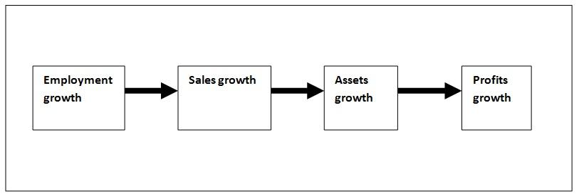
Figure 1: Growth processes: full sample (and subsample of non-HGFs).
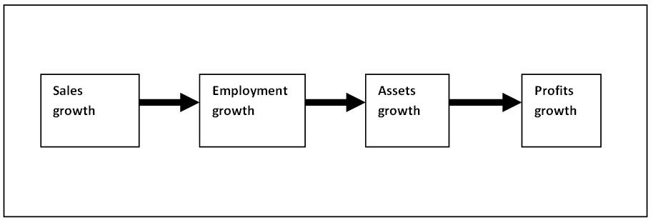
Figure 2: Growth processes: subsample of HGFs.
the possibility that it is anticipated profits that is driving the process of firm growth. We cannot tell whether managers seek to maximize anticipated profits as opposed to growth, because we don't have data on anticipated profits.
HGFs and rivalry In our peer-effects regressions, we investigated the complementarity of HGFs with other firms. Should HGFs be seen as 'cannibals' or 'parasites', that merely take up growth opportunities that would probably otherwise have been built upon by other firms? Do HGFs hastily botch growth opportunities that might be better exploited by other, more patient firms? Or do they play a complementary role in product and factor markets, helping to create new markets that other firms can also serve? Our results suggest that the growth of HGFs is similar, in terms of the rivalrous nature of their growth, to the growth of other firms. This result can be taken as encouraging, because it suggests that HGFs play a complementary role in the wider ecology of firms (in the sense that they are not especially ‘predatory' or ‘cannibalistic'). Our insights into the interdependence of HGF growth and the growth of other firms is related to some previous findings about how HGFs contribute to the wider economy. Coad et al. (2011a) look at matched employer-employee data for Swedish HGFs, and find that HGFs seem to employ those individuals that are relatively marginalized on the labour market (such as the young, immigrants, the unmarried, and those who have experienced longer spells in unemployment and self-employment). It is also worth mentioning that Bos and Stam (2011) observe that an increase in the presence of HGFs in an industry contributes to subsequent industry growth, whereas the reverse causal direction seems to be weaker (that is, less of an effect of industry growth on subsequent number of HGFs).
References
Achtenhagen, L., Naldi, L., and Melin, L. (2010). “Business Growth” – Do Practitioners and Scholars Really Talk About the Same Thing? Entrepreneurship theory and practice, 34(2):289–316.
Audretsch, D., Prince, Y., and Thurik, A. (1999). Do small firms compete with large firms? Atlantic Economic Journal, 27(2):201–209.
Bos, J. and Stam, E. (2011). Gazelles, industry growth, and structural change. Discussion Paper Series 11-02, Utrecht School of Economics.
Bramoullé, Y., Djebbari, H., and Fortin, B. (2009). Identification of peer effects through social networks. Journal of Econometrics, 150(1):41–55.
Caves, R. (1998). Industrial organization and new findings on the turnover and mobility of firms. Journal of Economic Literature, 36(4):1947–1982.
Coad, A. (2007a). A closer look at serial growth rate correlation. Review of Industrial Organization, 31(1):69–82.
Coad, A. (2007b). Testing the principle of 'growth of the fitter': the relationship between profits and firm growth. Structural Change and Economic Dynamics, 18(3):370-386.
Coad, A. (2009). The Growth of Firms: A Survey of Theories and Empirical Evidence. Edward Elgar: Cheltenham, UK.
Coad, A. (2010). Exploring the processes of firm growth: evidence from a vector autoregression. Industrial and Corporate Change, 19(6):1677–1703.
Coad, A., Daunfeldt, S., Johansson, D., and Wennberg, K. (2011a). Who do high-growth firms employ, and who do they hire? RATIO working papers, RATIO Institute, Stockholm.
Coad, A., Rao, R., and Tamagni, F. (2011b). Growth processes of Italian manufacturing firms. Structural Change and Economic Dynamics, 22(1):54–70.
Coad, A. and Teruel, M. (2012). Inter-firm rivalry and firm growth: Is there any evidence of direct competition between firms? Industrial and Corporate Change, forthcoming. doi:10.1093/icc/dts018.
Coad, A. and Valente, M. (2011). Hunting for a bogeyman? in search of statistical evidence of direct competition between firms. Evolutionary and Institutional Economics Review, 8(1):65–85.
Cowling, M. (2004). The growth-profit nexus. Small Business Economics, 22(1):1–9.
Davezies, L., D'Haultfoeuille, X., and Fougère, D. (2009). Identification of peer effects using group size variation. Econometrics Journal, 12(3):397–413.
Evans, P. and Welpton, R. (2009). Methods explained – business structure database. Economic and Labour Market Review, 3(6):71–75.
Fisher, F. and McGowan, J. (1983). On the misuse of accounting rates of return to infer monopoly profits. American Economic Review, 73(1):82–97.
Geroski, P. A. (2000). The growth of firms in theory and practice. In Foss, N. and Mahnke, V., editors, Competence, Governance, and Entrepreneurship. Oxford University Press, Oxford, UK.
Geroski, P. A. and Gugler, K. (2004). Corporate growth convergence in Europe. Oxford Economic Papers, 56:597–620.
Henrekson, M. and Johansson, D. (2010). Gazelles as job creators: a survey and interpretation of the evidence. Small Business Economics, 35(2):227–244.
Hölzl, W. (2011). Persistence, survival and growth: A closer look at 20 years of high growth firms in austria. Paper presented at the RATIO Institute workshop on High Growth Firms, Stockholm, Sweden.
Hoyer, P., Shimizu, S., and Kerminen, A. (2006). Estimation of linear, non-gaussian causal models in the presence of confounding latent variables. Proceedings of the Third European Workshop on Probabilistic Graph Models (PGM 06), pp155-162. Available as Arxiv preprint cs/0603038.
Hyvärinen, A., Karhunen, J., and Oja, E. (2001). Independent component analysis, volume 26. Wiley-interscience.
Hyvärinen, A., Zhang, K., Shimizu, S., and Hoyer, P. (2010). Estimation of a structural vector autoregression model using non-gaussianity. Journal of Machine Learning Research, 11:1709–1731.
Lacerda, G., Spirtes, P., Ramsey, J., and Hoyer, P. (2008). Discovering cyclic causal models by independent components analysis. Proceedings of the 24th Conference on Uncertainty in Artificial Intelligence (UAI-2008).
Lee, L. (2007). Identification and estimation of econometric models with group interactions, contextual factors and fixed effects. Journal of Econometrics, 140(2):333–374.
Manski, C. (1993). Identification of endogenous social effects: The reflection problem. Review of Economic Studies, 60(3):531–542.
Mason, C. and Brown, R. (2010). High Growth Firms in Scotland. Final report for Scottish Enterprise: Glasgow.
McKelvie, A. and Wiklund, J. (2010). Advancing firm growth research: A focus on growth mode instead of growth rate. Entrepreneurship theory and practice, 34(2):261-288.
Moneta, A., Chlaß, N., Entner, D., and Hoyer, P. (2011). Causal search in structural vector autoregressive models. Journal of Machine Learning Research: Workshop and Conference Proceedings, 12:95–114.
Moneta, A., Entner, D., Hoyer, P., and Coad, A. (2012). Causal inference by independent component analysis: Theory and applications. Oxford Bulletin of Economics and Statistics, Forthcoming. DOI: 10.1111/j.1468-0084.2012.00710.x.
Nickell, S. (1996). Competition and corporate performance. Journal of political economy, 104(4):724–746.
Oberhofer, H. and Pfaffermayr, M. (2010). Firm growth in multinational corporate groups. Working Paper no. 2010-07, University of Salzburg.
Parker, S., Storey, D., and van Witteloostuijn, A. (2010). What happens to gazelles? The importance of dynamic management strategy. Small Business Economics, 35:203–226.
Penrose, E. T. (1959). The Theory of the Growth of the Firm. Basil Blackwell, Oxford.
Shimizu, S., Hoyer, P., Hyvärinen, A., and Kerminen, A. (2006). A linear non-gaussian acyclic model for causal discovery. Journal of Machine Learning Research, 7:2003–2030.
Stone, J. (2004). Independent component analysis: a tutorial introduction. MIT Press, Cambridge, MA.
Storey, D. (1994). Understanding the small business sector. Thomson, London, UK.
Sutton, J. (1997). Gibrat's legacy. Journal of Economic Literature, XXXV:40–59.
Sutton, J. (2007). Market share dynamics and the 'persistence of leadership' debate. American Economic Review, 97(1):222–241.
Wiklund, J. (2007). Small firm growth strategies. In Zackarakis, A. and Spinelli, S., editors, Entrepreneurship and growth: The engine of Growth (2nd edition), chapter 7, pages 135-154. Praeger: Westport, Connecticut.
Appendices
A. Databases used
|
BSD |
FAME |
| Data coverage: firms |
Comprehensive coverage of all except micro firms |
Good coverage of large firms |
| Data coverage: years |
Good: We focus on 1998-2008 |
Good: We focus on 2003-2011 |
| Minimum size threshold |
VAT registration threshold; employer firms |
Companies that must file annual statements (listed firms, limited companies, etc) |
| Data source |
VAT records, National Insurance files |
Companies House files |
| Access for researchers |
Confidential/restricted access |
Publicly available (for a fee) |
| Number of variables |
Few |
Many (but with many gaps) |
| Variables |
Sales, employment, industry, region, etc. |
Sales, employment, financial variables, firm ID, and many others |
| Software limitations |
Limited |
Relatively easy to apply new software |
| Location in our paper |
Section 2 |
Sections 3-5 |
Table A.1: Comparison of the UK databases used in this paper.
B. SVAR methodology
B.1. Methodology
Consider the following Structural Vector Autoregression (SVAR) model:
$$
Y_t = B y_t + \Gamma_1 y_{t-1} + \dots + \Gamma_p y_{t-p} + \mathcal{E}_t, \quad \text{(3)}
$$
where the vector $y_t$ is a $m \times 1$ vector of dependent variables, where m=4 in our application and corresponds to the four variables sales growth, employment growth, assets growth and the profit margin, respectively. $\Gamma_p$ is the $m \times m$ matrix of coefficients on the p-th lag of y. Of central interest in SVAR models to our analysis is the matrix B, which denotes the ‘instantaneous' causal effects of one variable on another, that occur within the same time period $t$. B is defined as having a zero diagonal. Equation (3) is clearly endogenous, because $y_t$ appears on both sides of the equation.
This equation can be rewritten by making $y_t$ appear on the left hand side only, which yields the following reduced-form Vector Autoregression model:
$$
\begin{aligned}
y_t &= (I - B)^{-1}\Gamma_1 y_{t-1} + \dots + (I - B)^{-1}\Gamma_p y_{t-p} + (I - B)^{-1}\mathcal{E}t \
&= A_1 y
\end{aligned}
$$} + \dots + A_p y_{t-p} + u_t, \quad \text{(4)
Equation (4) can be estimated using conventional estimators such as OLS. The coefficient estimates for $A_i$ in Equation (4) describe the lead-lag relationships between the variables over time, although they do not provide estimates of instantaneous effects between variables, and hence do not describe the causal mechanisms between variables. In algebraic terms, Equation (4) essentially confounds the instantaneous causal effects B with the lagged effects Γ. As such, reduced-form VARs are suitable for describing the evolution of a system over time, but are mute with regards to the causal relations driving the system.
In order to uncover the matrix of causal effects B, we will need a different approach. In the literature on structural VARs (SVARs), one way of identifying B is by imposing the causal structure a priori by referring to economic theory. This is unsatisfactory, however, if theory is not sufficiently clear. Another approach is the graph-theoretic approach, but not sufficient to reveal all possible causal mechanisms. We take a relatively new approach, using Independent Components Analysis to identify a set of independent latent shocks, that are then ordered in an acyclic causal ordering to obtain estimates of B and Γ.
As shown in Equation (4), we have $u_t = (I – B)^{-1}\mathcal{E}_t$, where $(I – B)^{-1}$ is a square matrix (Moneta et al., 2011). The assumption of acyclicity guarantees that the matrix $(I – B)$ is invertible (Hyvärinen et al., 2010). To identify the matrix of instantaneous effects B, we analyse the reduced-form VAR residuals $u_t$ and apply Independent Component Analysis (ICA). In the next subsection, we present the intuition behind ICA, before providing details on how ICA is used as a key step in our algorithm for obtaining estimates for B in the context of a Structural VAR.
B.2. The intuition of ICA
Figure B.1 aims to clarify the intuition behind Independent Component Analysis as a tool for recovering the latent, statistically independent, source signals from data on the signal mixtures. The example in Figure B.1, based on Stone (2004), relates to the human voice, which is a high kurtosis signal. Two individuals are standing in a room with two microphones, and they both speak at the same time. The microphones record a mixture of both voices, although each microphone gives different weights to each voice – this is because the microphones are placed at different points in the room. Each microphone can be taken as being ‘closest' to one of the voices even though it will be a mixture of both voices. As high kurtosis signals are mixed together, Central Limit Theorem (CLT) implies that the mixture distribution will be more Gaussian than the source signals taken individually.
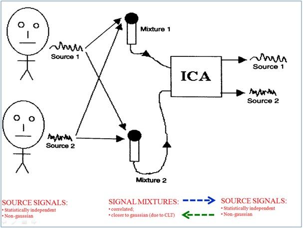
Figure B.1: Source signals (statistically independent) are mixed together and become more Gaussian (via central limit theorem) as they are recorded as signal mixtures. We attempt to recover the original source signals by performing ICA (and hence maximizing non-Gaussianity) on the observed signal mixtures, to generate a set of independent, non-Gaussian estimates for the source signals. Based on Stone (2004, p. 6).
Figure B.1 can be useful to give a first idea of how ICA is used, although the analogy is not perfect. Figure B.1 suggests a cyclic structure (each of the Sources affects each of the Mixtures) whereas in our model we assume an acyclic structure, which means that, in one case, we have Source$_i$ = Mixture$_i$, where $i$ = 1 or 2 or 3 or 4.
B.3. Identification strategy
Our identification strategy involves the following eight steps of the VAR-LINGAM 'recipe' (following Moneta et al., 2012):
- Estimate the reduced form VAR model of equation (4), obtaining estimates $\hat{A}\tau$ of the matrices $A\tau$, for $\tau = 1, \dots, p$. Denote by $\hat{U}$ the $K \times T$ matrix of the corresponding estimated VAR error terms, that is each column of $\hat{U}$ is $\hat{u}t \equiv (\hat{u}}, \dots, \hat{u{Kt})'$, ($t = 1, \dots, T$). Check whether the $\hat{u}$ (for all rows $i$) indeed are non-Gaussian, and proceed only if this is so.
- Use FastICA or any other suitable ICA algorithm (Hyvärinen et al., 2001) to obtain a decomposition $\hat{U} = P\hat{E}$, where P is $K \times K$ and $\hat{E}$ is $K \times T$, such that the rows of $\hat{E}$ are the estimated independent components of $\hat{U}$. Then validate non-Gaussianity and (at least approximate) statistical independence of the components before proceeding.
- Let $\hat{\Gamma}0 = P^{-1}$. Find $\tilde{\Gamma}_0$, the row-permuted version of $\hat{\Gamma}_0$ which minimizes $\sum_i 1/|\tilde{\Gamma}|$ with respect to the permutation. Note that this is a linear matching problem which can be easily solved even for high K (Shimizu et al., 2006).
- Divide each row of $\tilde{\Gamma}_0$ by its diagonal element, to obtain a matrix $\tilde{\Gamma}_0$ with all ones on the diagonal.
- Let $B = I – \tilde{\Gamma}_0$.
- Find the permutation matrix Z which makes $ZBZ^T$ as close as possible to strictly lower triangular. This can be formalized as minimizing the sum of squares of the permuted upper-triangular elements, and minimized using a heuristic procedure (Shimizu et al., 2006). Set the upper-triangular elements to zero, and permute back to obtain B which now contains the acyclic contemporaneous structure. (Note that it is useful to check that $ZBZ^T$ indeed is close to strictly lower-triangular.)
- B now contains $K(K – 1)/2$ non-zero elements, some of which may be very small (and statistically insignificant). For improved interpretation and visualization, it may be desired to prune out (set to zero) small elements at this stage, for instance using a bootstrap approach. See Shimizu et al. (2006) for details.
- Finally, calculate estimates of $\hat{\Gamma}\tau$, $\tau = 1, \dots, p$, for lagged effects using $\hat{\Gamma}\tau = (I – B)\hat{A}_\tau$.
B.4. Assumptions of the estimator
The main assumption required by our VAR-LiNGAM estimator is that the SVAR residuals $\mathcal{E}_t$ are non-Gaussian. This assumption cannot be tested directly, although we can check that the related VAR residuals $u_t$ are non-Gaussian. In line with a large literature on firm growth, these growth rate residuals are highly non-Gaussian.
The estimator also assumes that the causal structure is acyclic – that there is one main direction of causality between variables, and that feedback loops are not predominant. The assumption of acyclicity allows us to uniquely connect the SVAR shocks $\mathcal{E}_t$ to the components of $u_t$ in order to fully identify the causal structure (Moneta et al., 2011). The assumption of acyclicity is instrumental in step 6 of the aforementioned algorithm, where the permutation matrix Z is used to make $ZBZ^T$ as close as possible to strictly lower triangular, by minimizing the sum of squares of the permuted upper-triangular elements. In practical terms, the assumption of acyclicity is satisfied by rearranging the matrix B such that the major causal directions are given more importance, while relatively minor causal channels are assumed to be approximately equal to zero. The trick is to rearrange the matrix B to make the acyclicity assumption as realistic as possible. While we consider this approximation to be sufficiently plausible for our present purposes, we nonetheless eagerly await further developments in SVAR modelling that allows for cyclic causal relations.
Our VAR-LINGAM model also assumes that each VAR residual $u_t$ is primarily attached to one of the SVAR residuals $\mathcal{E}_t$. In terms of the intuition in Figure B.1, each microphone is ‘closest' to one of the voices. In terms of Figure B.2, each independent component $\mathcal{E}_t$ is more closely associated with the corresponding residual $u_t$, although of course we allow for the possibility that each $\mathcal{E}_t$ is also related in some way to each other $u_t$. This assumption will be useful as we seek to put the source signals (‘voices') into a causal order using information gathered from the signal mixtures ('microphones').
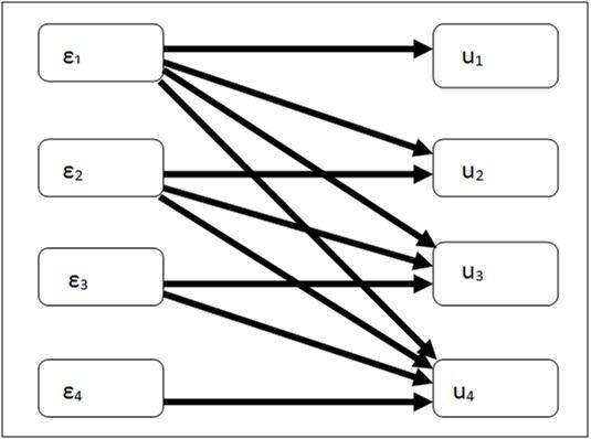
Figure B.2: Stylised representation of the lower-diagonal matrix P from the expression $\hat{U} = P\hat{E}$ (Step 2 of our identification strategy). The $\mathcal{E}_t$ correspond to the independent components, while the $u_t$ correspond to the observed residuals.
Three other assumptions can be named here, that are shared with more conventional regression estimators. The first concerns omitted variable bias – it is assumed that there are no strong confounding variables that have been omitted from the VAR system. Second, VAR-LiNGAM is a linear regression model, which assumes that the relationships between the dependent and explanatory variables are linear. In view of previous work on firm growth, this assumption seems reasonable. Third, the SVAR shocks $\mathcal{E}_t$ are assumed to be independent – that is, independent across VAR series, and independent over time. This seems to be a reasonable assumption in our present context, especially considering that the SVAR shocks are independent by construction due to our ICA process.
C. Quantile-quantile plots
![A grid of eight statistical plots, including four histograms of X[, i] on the top row and four Normal Q-Q Plots on the bottom row, displaying data distributions and normality.](https://media.nesta.org.uk/images/page_39_img_0_FrkJNw4.original.jpg)
Figure C.3: Analysis of the residuals of a 1-lag VAR. The four columns correspond to the distributions of sales growth, employment growth, growth of total assets and growth of profit margin. The top row presents histograms of the residuals with a fitted Gaussian (same mean and variance). The bottom row presents quantile-quantile plots of the residuals, plotted against a Gaussian. These plots follow Moneta et al. (2012).
D. Peer-effects methodology
Consider the following regression equation:
$$
g_{ir} = \lambda \cdot \frac{1}{m_r - 1} \sum_{j \neq i}^r g_{jr} + \gamma X_{ir} + \mu_r + \epsilon_{ir} \quad \text{(5)}
$$
where $g_{ir}$ is the growth rate of firm $i$ in group $r$, $X_{ir}$ corresponds to a set of exogenous control variables (i.e. lagged size, and industry growth). Previous work on firm growth suggests that these two variables are among the most important factors affecting firm growth (Coad, 2009), although it is notoriously difficult to find the determinants of firm growth because firm growth seems to be a predominantly random process (Geroski, 2000). (This implies we need not be especially concerned with omitted variable bias in our present context.) In our application, the parameter of interest is $\lambda$, which indicates how a firm's growth is influenced by the growth of its rivals. $m_r$ corresponds to the 'group size'; that is, number $m$ of firms in sector $r$. $\mu_r$ is a group-specific fixed effect (that is, a time-invariant sector-specific effect).
The econometric issue is that the growth of rival firms may simultaneously affect each other – a firm's growth may be limited by the growth of its rival, at the same time as the rival's growth is affected by the growth of the first firm. This problem has been called the 'reflection problem' by Manski (1993), because “the problem is similar to that of interpreting the almost simultaneous movements of a person and his reflection in a mirror" (Manski, 1993, p. 532).
Equation (5) can be rewritten as:
$$
g_{ir} = \frac{\lambda}{m_r - 1}(m_r \bar{g}r – g
$$}) + \gamma X_{ir} + \mu_r + \epsilon_{ir} \quad \text{(6)
Taking averages across groups, we obtain the between-group equation:
$$
\bar{g}_r = \frac{\lambda}{m_r - 1}(m_r \bar{g}_r - \bar{g}_r) + \gamma \bar{X}_r + \mu_r + \bar{\epsilon}_r \quad \text{(7)}
$$
which can be rearranged to yield:
$$
\bar{g}_r = \frac{1}{1 - \lambda}(\gamma \bar{X}_r + \mu_r + \bar{\epsilon}_r) \quad \text{(8)}
$$
Subtracting (8) from (6) yields:
$$
(g_{ir} - \bar{g}r) = -\lambda \frac{(g}-\bar{gr)}{(m_r - 1)} + \gamma(X} - \bar{Xr) + (\epsilon
$$} - \bar{\epsilon}_r) \quad \text{(9)
Equation (9) is to the within-group equation, in which an individual firm's growth is related to the average growth of the rival firms in the same sector. As emphasized by Oberhofer and Pfaffermayr (2010), the peer-effect parameter $\lambda$ cannot be identified in the between-group equation (7), but instead it must be identified using the within-group equation (9).
Note that the dependent variable is the term $(g_{ir} – \bar{g}r)$, which is different from the dependent variable that appears in conventional regressions, and this implies that care should be taken in comparing our regression results with those obtained in other work. The first term on the right-hand side is clearly endogenous – $g$, where the tilde ‘~' denotes an estimated value) to derive an improved instrument, that we use in another 2SLS estimation of equation (9).}$ has an influence on $g_{jt}$, but $g_{jt}$ also influences $g_{it}$. To deal with this endogeneity, we apply instrumental-variable (IV) techniques (following Oberhofer and Pfaffermayr (2010)), which involves two iterative instances of instrumental variable (IV) estimation. First, we use the exogenous variables multiplied by $\frac{1}{(m_r-1)}$ as instruments in a two-stage least squares (2SLS) regression of equation (9) to obtain a consistent initial estimator of $\lambda$. Second, we use this estimate of $\lambda$ (i.e. $\tilde{\lambda In this second stage, we introduce dummies for HGFs to distinguish the growth experiences of HGFs vs non-HGFs. Therefore, we use information from the whole group to estimate the rivalry coefficient $\lambda$, but report the rivalry coefficient $\lambda$ as it corresponds to subsamples of HGFs or non-HGFs.
Bearing in mind that $\frac{(g_{ir}-\bar{g}r)}{(m_r-1)}$ can be rearranged to yield $\frac{(g}-\bar{gr) + \lambda \frac{(g}-\bar{gr)}{(m_r-1)}}{ (m_r-1)}$, we use our first-stage IV estimates (that is, the predicted values) to instrument $\frac{(g$ by the following term:}-\bar{g}_r)}{(m_r-1)
$$
\frac{(g_{ir} - \bar{g}r) + \tilde{\lambda} \frac{(g
$$} - \bar{g}_r)}{(m_r - 1)}}{ (m_r - 1 + \tilde{\lambda})} \quad \text{(10)